or \[ b_{63}~b_{62} \dotsc b_{52}~b_{51}\dotsc b_{0} \] where
We are going to be mostly interested in working with numbers. Specifically, integers (\(\mathbb{N}, \mathbb{Z}\)), real numbers (\(\mathbb{R}\))
Design constraints:
Finite storage
physical representation needs to be encoded using 0/1
Some terminology:
Bit : basic unit of representation - can be either 0 or 1
Byte : 8 bits. Usually the smallest unit that we can work with
Motivation: How does the decimal system work?
Non-negative Integers: \(\sum_{i=0}^{n-1} d_i \times 10^i = d_{n-1} d_{n-2} \ldots d_1 d_0\)
Signed integers: Same as above, along with a sign
Fractions (between 0 and 1): \(\sum_{i=1}^{n} d_i \times 10^{-i} = 0.d_1 s_2 d_{n-1} d_{n}\)
General real numbers: \(\sum_{i=-m}^{n} d_i \times 10^{i}\)
Can we adapt this to use binary digits? Not very difficult for integers:
We can see examples in Julia:
julia> bits(20)
"0000000000000000000000000000000000000000000000000000000000010100"

julia> bits(convert(Uint8, 20))
"00010100"

julia> [bits(convert(Uint8, x)) for x = [1, 2, 3, 4, 5, 6, 7, 8, 9, 10]]
10-element Array{ASCIIString,1}:
 "00000001"
 "00000010"
 "00000011"
 "00000100"
 "00000101"
 "00000110"
 "00000111"
 "00001000"
 "00001001"
 "00001010"
Clearly, we can only store a finite number of integers using this representation (specifically, \(2^n\)).
julia> typemin(Uint8)
0x00

julia> typemax(Uint8)
0xff

julia> bits(typemax(Uint8))
"11111111"
Numbers prefixed with 0x means hexadecimal coding (with digits 0123456789abcdef meaning 0--16).
How can we add two numbers? Simply add bit by bit, with 1 + 1 = 0 carrying 1, and 1 + 1 + 1 = 1 carrying 1.
 111

001110 +   (14)
000111 =   (07)

010101     (21)
What happens if we add 1 to the maximum possible value?
function addone(x::Uint8)
    y::Uint8 = x + convert(Uint8, 1)
    y
end

julia> bits(addone(convert(Uint8, 3)))
"00000100"

julia> bits(addone(typemax(Uint8)))
"00000000"
This is known as "overflow". For efficiency (to minimize time needed to do checking), many systems will silently overflow without informing the user that something might have gone wrong.
How do we store signed integers?
By convention, the first (leftmost) bit is used for the sign
In addition, negative numbers are stored using a convention known as "two's complement", which basically stores an \(N-1\)-bit negative number as its complement w.r.t. \(2^N\), i.e., the result of subtracting the number from \(2^N\)
Advantages: addition, multiplication, etc. can be performed using the same algorithm as unsigned integers. Also, zero has a unique representation, so \(2^N\) distinct numbers can be stored.
julia> [bits(convert(Int8, x)) for x = [-10:10]]
21-element Array{ASCIIString,1}:
 "11110110"
 "11110111"
 "11111000"
 "11111001"
 "11111010"
 "11111011"
 "11111100"
 "11111101"
 "11111110"
 "11111111"
 "00000000"
 "00000001"
 "00000010"
 "00000011"
 "00000100"
 "00000101"
 "00000110"
 "00000111"
 "00001000"
 "00001001"
"00001010"Numerical computations usually require working with "real numbers". Motivated by the decimal representation of real numbers, we can think of them as binary numbers of the form \[ b_1 b_2 \dotsc b_k [.] b_{k+1} \dotsc b_n \] which we could perhaps store as the pair \((b_1 \dotsc b_n, k)\). This is actually fairly close to what we do in practice. The numbers that can be represented exactly have the form \[ significand \times base^{exponent} \] For example, \[ 1.2345 = 12345 \times 10^{-4} \] or with base=2 and binary digits, \[ 110.1001 = 1.101001 \times 2^{10} \] This is known as the floating point representation.
We still need to decide how to store the significand and the exponent. Modern computers have two standard storage conventions for floating point representations:
32-bit : known as single precision/float/Float32
64-bit : known as double precision/double/Float64
The conventions are detailed in the IEEE 754 standard, and is summarized in the following table.
| Float32 | Float64 | |
|---|---|---|
| sign | 1 | 1 |
| exponent | 8 | 11 |
| fraction | 23 (+1) | 52 (+1) |
| total | 32 | 64 |
| exponent offset | -127 | -1023 |
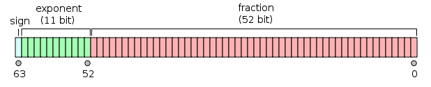
For example, bits in a Float64 is laid out in the following way:
or \[
b_{63}~b_{62} \dotsc b_{52}~b_{51}\dotsc b_{0}
\] where
\(s = b_{63}\) is the sign bit,
\(e = b_{62}\dotsc b_{52}\) is the exponent interpreted as an 11-bit unsigned integer,
and the number represented is calculated as \[ (-1)^s (1.b_{51}\dotsc b_{0}) \times 2^{e-1024} \] Note that the fraction has an implicit 1 before the binary point that is not explicitly stored. This is a form of "normalization" that ensures uniqueness of the representation, and implicitly allows an extra bit of precision.
The minimum (0) and maximum (2047) possible value of \(e\) are reserved for special use, and cannot be used as above. They are used as representations for special numbers \(\pm \infty\), NaN, \(\pm 0\), and "subnormal" numbers between 0 and \(1.0 \times 2^{-1023}\) (the smallest positive number that would have been representable had \(e=0\) been allowed with the usual interpretation).
julia> bits(0.1)
"0011111110111001100110011001100110011001100110011001100110011010"

julia> bits(0.1 + 0.1 + 0.1)
"0011111111010011001100110011001100110011001100110011001100110100"

julia> bits(0.3)
"0011111111010011001100110011001100110011001100110011001100110011"

# 0 and subnormal numbers (e = 0)
julia> bits(0.0)
"0000000000000000000000000000000000000000000000000000000000000000"

julia> bits(-0.0)
"1000000000000000000000000000000000000000000000000000000000000000"

julia> bits(0.125 * 1.0 * 2.0^(-1023))
"0000000000000001000000000000000000000000000000000000000000000000"

# Inf and NaN (e = 2047)
julia> bits(Inf)
"0111111111110000000000000000000000000000000000000000000000000000"

julia> bits(-Inf)
"1111111111110000000000000000000000000000000000000000000000000000"

julia> bits(NaN)
"0111111111111000000000000000000000000000000000000000000000000000"
Note in the above example that 0.1 + 0.1 + 0.1 has a different representation than 0.3. This is because the binary representation of 0.1, 0.2, 0.3, etc. are recurring, and cannot be represented exactly. When represented as floating point numbers, they need to be approximated (ideally by the nearest representable number, though this may not always happen in practice). So depending on intermediate calculations, results that are supposed to be the same may not be.
julia> 0.2 + 0.1 == 0.4 - 0.1
true

julia> 0.2 + 0.1 == 0.6 / 2
false

julia> 0.2 + 0.1
0.30000000000000004
Note that in the representation (of what is supposed to be 0.3) is an approximation in all cases, and the question is only whether two approximations derived at differently agree or not.
The same behaviour is seen in python
>>> 0.2 + 0.1 == 0.4 - 0.1
True
>>> 0.2 + 0.1 == 0.6 / 2
False
>>> 0.2 + 0.1
0.30000000000000004
and R
> 0.2 + 0.1 == 0.4 - 0.1
[1] TRUE
> 0.2 + 0.1 == 0.6 / 2
[1] FALSE
> 0.2 + 0.1
[1] 0.3
except that R tries to be "user-friendly" and rounds the result before printing (to 7 digits by default).
> print(0.2 + 0.1, digits = 22)
[1] 0.3000000000000000444089In the case of integer calculations, unreported overflow is the most common problem. For example, in Julia, defining:
function Factorial(x)
    if (x == 0) tmp = 1
    else tmp = x * Factorial(x-1)
    end
    println(tmp)
    tmp
end
we get
julia> Factorial(25)
1
1
2
6
24
120
720
5040
40320
362880
3628800
39916800
479001600
6227020800
87178291200
1307674368000
20922789888000
355687428096000
6402373705728000
121645100408832000
2432902008176640000
-4249290049419214848
-1250660718674968576
8128291617894825984
-7835185981329244160
7034535277573963776

julia> Factorial(25.0)
1
1.0
2.0
6.0
24.0
120.0
720.0
5040.0
40320.0
362880.0
3.6288e6
3.99168e7
4.790016e8
6.2270208e9
8.71782912e10
1.307674368e12
2.0922789888e13
3.55687428096e14
6.402373705728e15
1.21645100408832e17
2.43290200817664e18
5.109094217170944e19
1.1240007277776077e21
2.585201673888498e22
6.204484017332394e23
1.5511210043330986e25
R behaves similarly, except that it detects integer overflow (the 1L in the code is to force integer calculations when x is integer; in R the literal 1 is interpreted as a floating point value and 1L as integer).
Factorial <- function(x) {
    if (x == 0) {
        tmp <- 1L
    }
    else {
        tmp <- x * Factorial(x-1L)
    }
    print(tmp)
    tmp
}
gives
> Factorial(15L)
[1] 1
[1] 1
[1] 2
[1] 6
[1] 24
[1] 120
[1] 720
[1] 5040
[1] 40320
[1] 362880
[1] 3628800
[1] 39916800
[1] 479001600
[1] NA
[1] NA
[1] NA
[1] NA
Warning message:
In x * Factorial(x - 1L) : NAs produced by integer overflow
> Factorial(25.0)
[1] 1
[1] 1
[1] 2
[1] 6
[1] 24
[1] 120
[1] 720
[1] 5040
[1] 40320
[1] 362880
[1] 3628800
[1] 39916800
[1] 479001600
[1] 6227020800
[1] 87178291200
[1] 1.307674e+12
[1] 2.092279e+13
[1] 3.556874e+14
[1] 6.402374e+15
[1] 1.216451e+17
[1] 2.432902e+18
[1] 5.109094e+19
[1] 1.124001e+21
[1] 2.585202e+22
[1] 6.204484e+23
[1] 1.551121e+25
[1] 1.551121e+25
Python has more interesting behaviour, because it detects integer overflow and automatically shifts to using a less efficient but higher precision representation.
def Factorial(x):
    if x == 0:
        tmp = 1
    else:
        tmp = x * Factorial(x-1)
    print tmp
    return tmp
gives
>>> Factorial(25)
1
1
2
6
24
120
720
5040
40320
362880
3628800
39916800
479001600
6227020800
87178291200
1307674368000
20922789888000
355687428096000
6402373705728000
121645100408832000
2432902008176640000
51090942171709440000
1124000727777607680000
25852016738884976640000
620448401733239439360000
15511210043330985984000000
15511210043330985984000000L
>>> Factorial(25.0)
1
1.0
2.0
6.0
24.0
120.0
720.0
5040.0
40320.0
362880.0
3628800.0
39916800.0
479001600.0
6227020800.0
87178291200.0
1.307674368e+12
2.0922789888e+13
3.55687428096e+14
6.40237370573e+15
1.21645100409e+17
2.43290200818e+18
5.10909421717e+19
1.12400072778e+21
2.58520167389e+22
6.20448401733e+23
1.55112100433e+25
In practice, numerical calculations are done using floating point arithmetic, where possible problems are more subtle.
One obvious limitation is that although floating point numbers can represent numbers of much larger magnitude, only the first few significant digits are actually stored. So, in all the examples above, we get something like
> x = factorial(25.0)
> x
[1] 1.551121e+25
> x == x + 1
[1] TRUE
The essential point is that given a value, how far away the closest representable value is depends on the value. In Julia, eps(x) returns a value such that x + eps(x) is the next representable floating-point value larger than x.
julia> eps(1.0)
2.220446049250313e-16

julia> eps(1000.)
1.1368683772161603e-13

julia> eps(1e-27)
1.793662034335766e-43

julia> eps(0.0)
5.0e-324

julia> eps(1.5e+25)
2.147483648e9
Another extreme example of this behaviour is the following. Consider the mathematical identity \[ f(x) = 1 - \cos(x) = \sin^2(x) / (1 + cos(x)) \]
and suppose that we are interesting in evaluating \(f(x)\) for a given value of \(x\). In theory, we can use either formula. In practice, near \(x = 0\), \(\cos(x)\) is very close to 1, so \(1-\cos(x)\) loses precision.
f1 <- function(x) {
    1 - cos(x);
}
f2 <- function(x) {
    u <- sin(x);
    (u * u) / (1 + cos(x));
}
curve(f1, from = 0.0, to = 1e-7, n = 1001, col = "red")
curve(f2, from = 0.0, to = 1e-7, add = TRUE, n = 1001, col = "blue")Suppose \(x\) is approximately represented as \(x^*\). The difference \(x - x^*\) is the error in \(x^*\), and the corresponding relative error is \[ \frac{x - x^*}{x} \] Due to the nature of the floating point representation, it is the amount relative error inherent in the representation that is comparable across the range of representatable values. That is, multiplying \(x\) by a (large or small) constant will usually change the absolute error but not the relative error.
As we have seen before, relative error can be increased substantially by subtraction. That is, if \(x, y\) are close to each other but not close to 0, then \[ \left| \frac{(x-y) - (x-y)^*}{x-y} \right| >> \max ( |\frac{x-x^*}{x}|, |\frac{y-y^*}{y}| ) \] and more importantly, much larger than the relative error in \((x-y)^*\) inherent in the representation.
How can we study how errors propagate through various numerical calculations? This is studied in terms of the related concepts of condition (of a function) and instability (of a process to calculate a function).
Remark: Calculations are helped by noting that when the relative error is small, it can be approximated as \[ \frac{x-x^*}{x} \approx \frac{x-x^*}{x^*} \] (LHS / RHS = 1 - relative error).
Condition describes the sensitivity of a function \(f(x)\) to changes in \(x\). Roughly, the condition of \(f\) at \(x\) is \[ \max \left\lbrace \frac{ \left| \frac{f(x) - f(x^*)}{f(x)} \right| }{ \left| \frac{x-x^*}{x} \right|} : |x-x^*| \text{ is small} \right\rbrace = \max \left\lbrace \left| \frac{f(x) - f(x^*)}{x - x^*} \right| \cdot \left| \frac{x}{f(x)} \right| : |x-x^*| \text{ is small} \right\rbrace \approx \left| \frac{f'(x) x}{f(x)} \right| \] If the condition of \(f\) is large (at some \(x\)), we say \(f\) is "ill-conditioned" at \(x\).
Examples:
\(f(x) = \sqrt(x), x \geq 0\), \(f'(x) = \frac{1}{2} x^{-\frac{1}{2}}\). So the condition of \(f\) at \(x\) is \[ \left| \frac{f'(x) x}{f(x)} \right| = \frac{1}{2} \frac{x^{-\frac{1}{2}}}{x^\frac{1}{2}} x = \frac{1}{2} \] So \(f\) is well-conditioned for all \(x\).
\(f(x) = x^\alpha\). Condition of \(f\) is \(|\alpha|\) at all \(x\) (exercise).
\(f(x) = \frac{1}{1-x^2}\). \(f'(x) = 2x (1-x^2)^{-2}\). So condition of \(f\) at \(x\) is \[ \left| \frac{f'(x) x}{f(x)} \right| = \left| 2x (1-x^2)^{-2} x (1-x^2) \right| = \frac{2x^2}{|1-x^2|} \] which can be large for \(x\) close to \(\pm1\).
Instability describes the sensitivity of a process for calculating \(f(x)\) to the rounding errors that happen during calculation. The basic idea is to compare the condition of \(f(x)\) (which is inherent in \(f\)) with the conditions of the intermediate steps. Badly conditioned intermediate steps, for which the condition is much larger than the condition of \(f\), make the process unstable.
To make the idea concrete, suppose \(y = f(x)\) is computed in \(n\) steps. Let \(x_i\) be the output of the \(i\)th step (define \(x_0 = x\)). Then \(y=x_n\) can also be viewed as a function of each of the intermediate \(x_i\)s. Denote the \(i\)th such function by \(f_i\), such that \(y = f_i (x_i)\). In particular, \(f_0 = f\). Then the instability in the total computation is dominated by the most ill-conditioned \(f_i\). In other words, a computation is unstable if one or more of the \(f_i\)s have a condition much larger than the condition of \(f\).
Example: \(f(x) = \sqrt{x+1} - \sqrt{x}, x > 0\). It is easily seen that the condition of \(f\) at \(x\) is \(\frac{1}{2} \frac{x}{\sqrt{x+1} \sqrt{x}} \approx \frac{1}{2}\) for \(x\) large. Computing \(f\) directly from the definition will usually proceed as follows.
This defines \(f_i\)s as follows.
Consider the condition of \(f_3\), which is \[ \left| \frac{f_3'(t) t}{f_3(t)} \right| = \left| \frac{t}{x_2 - t} \right| \] This can be large (much larger than \(1/2\)) for large \(x\), e.g., in R
> x <- c(10, 100, 1000, 10000)
> abs(sqrt(x) / (sqrt(x+1) - sqrt(x)))
[1]    20.48809   200.49876  2000.49988 20000.49999
An alternative way to compute \(f(x)\) is as \(\frac{1}{\sqrt{x+1} + \sqrt{x}}\). This proceeds as
The corresponding \(f_i\)s are
All these have good condition when \(t\) is large (exercise).
There are many kinds of programs and many kinds of programming languages. We will mostly consider the procedural programming paradigm, which is an example of structured programming. The main features of this approach are
use of modular procedures (usually called functions)
use of various control flow structures
We will also be mainly interested in designing and writing procedures that perform computations, as opposed to interface programs whose main task is interacting with the user (such as an operating system, web browser, editor, etc.).
The main components of our programs are going to be functions. Usually a programming language will have some built-in functions, and additional libraries which will provide more standard functions. Functions usually
have one or more input arguments,
perform some computations, possibly calling other functions, and
return one or more output values.
The main contribution of a function is the second step, performing the computations. The standard model for this is a sequential execution of instructions. Some control flow structures may be used to create branches or loops in the sequence actually followed during the execution of a function. Briefly, the main ingredients used are:
Declaration of variables (implicit in some languages). The details of how variables store values, and who can access them (scope) are important, and will be discussed later.
Evaluation of expressions (involving variables that have previously defined).
Assignment to variables (to store intermediate results for later use).
Logical tests (equal?, less than?, greater than?, is more input available?).
Logical operations (AND, OR, NOT, XOR).
Branching - take different paths based on result of a logical operation (if then else).
Loops - repeat sequence of steps, usually a fixed number of times, or until a condition is satisfied (for, while).
Math: + - * / ^ %
Logical: & | !
Numeric comparisons: == != < > <= >=
Math functions: round, floor, ceil, abs, sqrt, exp, log, sin, cos, tan, asin, ...
These concepts are enough for us to start looking at some specific problems. Before writing an actual program, it is often useful to plan it out in a human-readable way. This is usually done using an algorithm, which is basically a step-by-step description of operations to be performed. Often, it is useful to graphically represent an algorithm using a diagram called a flow chart.
Here are some examples, specifically chosen not to need arrays (indexed vectors):
Compute factorial - direct, using log.
Compute \(n \choose k\).
Determine if a given number is a prime.
Simple symmetric random walk with \(\pm1\) steps - compute time of first return to 0.
How many times is a coin tossed until we get 2 consecutive heads?
An urn contains \(n\) black + \(n\) white balls. Pick balls without replacement, and let \(X_k\) = #black - #white after \(k\)th draw. What proportion of time is \(X_k > 0\)?
Some examples that need arrays and more general 'data structures':
The study of algorithms becomes interesting when we can find more than one way to solve a problem. Important questions are:
Is an algorithm correct? To be correct, an algorithm must stop (after a finite number of steps) and produce the correct output for all possible inputs (i.e., all instances of the problem).
How efficient is the algorithm? That is, how much resources the algorithm needs, typically in terms of time and storage.
We will study these questions mainly in the context of one specific problem, namely sorting.