Class projects

General guidelines

The purpose of class projects is two-fold. Their primary purpose is to evaluate you, but they are also intended to expose the whole class to certain important topics I will not cover separately. Keep this in mind when working on your projects.

For all projects, you should

• Submit a written report that will be put up on the course webpage.
• Prepare a presentation that summarizes your findings to the class. Your presentation should have enough details so that your audience gains a reasonable understanding of the problem you have tried to solve, the difficulties in solving it, and the solution(s) you have come up with.
• Wherever relevant, submit all code you have written. Your code should be well-formatted and commented, so that others can understand what it does without further explanation. (Unlike the Linear Models course, quality of code will count in grading.)
• For this course, the process of arriving at a solution is often more important than the solution itself. Do not hesitate to give details of your learning experience in your report and presentation.
• There are often many different ways to solve the same problem. Evaluating and comparing the different ways in an objective manner is an important skill. You are encouraged to try out various solutions and report on their relative merits. In particular, you should attempt to implement solution both in R and C/C++ whenever feasible and present a comparison.

Feel free to consult me if you have doubts regarding any of these requirements. If you need help doing the projects, you are free to seek help from me or anyone else who is willing to help (including other students in the class).

Set I

Project 1 (Kaustav, Gursharn, Smruti + Shwetab, Sagnika)

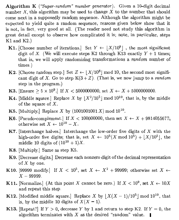
Present a brief history of random number generators as described in Knuth, The Art of Computer Programming (TAOCP), Vol 2. Describe and implement Von Neumann's squaring method (mentioned in class) and Algorithm K (given below). Use your implementation to verify and demonstrate the claims made about these generators.

For Von Neumann's method, implement a direct solution as well as a solution in C using the bitwise shift operators. Compare their performances. Also implement an interface that allows your generator to be used from R.

Briefly describe linear congruential generators and their properties.

Algorithm K is as follows.

Project 2 (Fadikar, Pinky + Arijit, Aurindam, Mansi)

Describe various tests for randomness of a sequence of pseudo-random numbers as described in TAOCP Vol 2. (Adjust your report and presentation keeping in mind that your audience knows statistics, unlike the target audience of the book.) Implement a reasonable subset of such tests. You do not need to implement the spectral test, but describe the idea behind it.

Write R code that takes a vector of (presumably random) numbers and produces an automated PDF report summarizing the results of these tests. Present the results of your tests applied on the various random number generators available in R (include a brief summary of what they are). See ?RNG for details.

Update: Here are two sets of 50000 pseudo-random numbers that you should also apply your tests on.

• Generated using Python's random module: numbers, code
• Generated using Javascript: numbers, webpage

Project 3 (Anujit, Pooja, Ipsita + Kanika, Eshita, Naveen)

Implement software to simulate a game of generalized snakes and ladders. The game is defined by a set of possible positions S = \{ 0, 1, 2, \ldots, N-1 \}, a set of snakes and ladders \{ (u_1, v_1), (u_2, v_2), \ldots, (u_m, v_m) \} where u_j \neq v_j \in S, and a k-sided die with probabilities p_1, p_2, \ldots, p_k. The game starts by setting the initial position X_1 = 0. At each step, a throw of the die determines the step size D_i which takes value j with probability p_j. If X_i + D_i = u_j for some j, then X_{i+1} = v_j, otherwise X_{i+1} = (X_i + D_i) \text{ mod } N . To make the game more interesting, we make it never-ending by making N equivalent to 0.

Your implementation should allow all the defining parameters to be specified by the user, but should use reasonable (perhaps random) defaults choices if not.

We are interested in the long-term behaviour (or asymptotic distribution) of X_i. Explore such behaviour using your program for various values of the parameters and summarize your observations.

Set II

Project 1 (Gursharn, Smruti)

Suppose we observe X \sim Bin(n, p). We are interested in confidence intervals for p. Compare the performance of (nominally) 95% confidence intervals obtained using

• The Normal approximation to Binomial
• Bootstrap-t
• Boostrap percentile

in terms of (1) length of the confidence interval and (2) observed coverage probability. Do this for

• n = 10, 20, 50, 100, 500, 1000, and
• p = 0.05, 0.1, 0.25, 0.5

Project 2 (Shwetab, Sagnika)

Let X_1, X_2, \ldots, X_n \sim i.i.d. F, \theta = F^{-1}(0.5). We are interested in confidence intervals for the population median based on the sample median. Compare the performance of (nominally) 95% confidence intervals obtained using

• The asymptotic Normal approximation (describe how you would obtain such an interval)
• Bootstrap-t
• Boostrap percentile

in terms of (1) length of the confidence interval and (2) observed coverage probability. Do this for

• n = 10, 20, 50, 100, 500, 1000, and
• F = Normal, Uniform, exponential, lognormal, t_5, and \chi_5^2.

Project 3 (Anujit, Pooja, Ipsita)

Consider the following regression models:

where \alpha = 1.5, \beta = 7.5, n = 15, x_i-s are generated from the U(0, 20) distribution, and \varepsilon_i-s are generated from one of the following distributions:

• Standard Normal
• t_5
• double exponential with rate 1
• logistic (with location parameter 0 and scale parameter 1)

Let \hat{\beta} be the OLS estimator of \beta. For each of the above cases, compare

• the true variance of \hat{\beta} (estimated)
• The estimated variance using delete-1 jackknife
• The estimated variance using residual bootstrap
• The estimated variance using paired bootstrap

Project 4 (Arijit, Aurindam, Kaustav)

(From C. R. Rao, LSI) Every human being can be classified nito one of four blood groups O, A, B, and AB. The inheritance of these blood groups is controlled by three allelomorphic genes O, A, B of which O is recessive to A and B. If r, p, q are gene frequencies of O, A, B respectively in the population, then the expected probabilities of the six genotypes (four phenotypes) in random mating are as follows

Genotype	Phenotype	Probability
OO	O	r^2
AA	A	p^2
AO	A	2pr
BB	B	q^2
BO	B	2qr
AB	AB	2pq

Phenotype	Probability
O	r^2
A	p^2 + 2pr
B	q^2 + 2qr
AB	2pq

Given observed counts n_O, n_A, n_B, n_{AB}, implement a program in C or C++ to compute the maximum likelihood estimates of p, q, r using the Fisher scoring method. In your presentation, give a brief background on the Newton-Raphson and Fisher scoring methods.

Project 5 (Fadikar, Pinky, Mansi)

For the same problem as project 4 above, write an R program to compute the MLE. You may find the following paper useful: http://www.jstor.org/stable/1390942. In your presentation, include a brief description of various numerical optimization methods available in R.

Set III

[This is the last set of projects. The project problems are not stated in as much detail as for the previous projects; please contact me for clarifications. ]

Project 1 (Gursharn, Smruti)

Derive the EM iteration for the problem of maximum likelihood estimation from a bivariate normal sample with some missing data. Implement your solution. Apply it on simulated data and comment on performance.

Project 2 (Shwetab, Sagnika)

Implement an EM algorithm to estimate parameters of a Normal mixture model. Apply it on simulated data and comment on performance.

Project 3 (Anujit, Pooja, Ipsita)

Implement the Baum-Welch algorithm to find MLEs for the occasionally dishonest casino example (assume that the probabilities of both dies are unknown). Apply it on simulated data and comment on performance (especially effect of sample size).

Project 4 (Arijit, Aurindam, Kaustav)

Show that the Richardson-Lucy algorithm is an example of the EM algorithm under a Poisson model for the observed intensity. Implement the algorithm and apply it on simulated examples.

Here is a test image (PNG version) that you can apply your algorithm on. The image was produced from the original by using a (suitably normalized) Gaussian point spread function f(x) = exp(-x^2/\sigma^2) with \sigma^2 = 10, where x is distance. The simplest way to get the image into R as a matrix is to use the pixmap package to read in the PGM file; e.g.,

library(pixmap)
lena <- read.pnm("lena_blurred.pgm")
str(lena@grey) ## matrix of values in [0, 1]

Project 5 (Fadikar, Pinky, Mansi)

Implement the Baum-Welch algorithm to find MLEs for a Hidden Markov Model with Gussian emission distributions with different means but common variance. Apply it on simulated data and comment on performance. Comment on the effect of model misspecification (number of states). Is the likelihood ratio test effective for choosing the correct number of states?

Optional: HMMs are a commonly used tool in speech recognition. A simpler but related problem is to process a piece of music to infer the underlying score (i.e., notation, sa-re-ga-ma, etc.). You can try to use your software for this purpose; contact me for further details if you are interested. (I have no idea how easy or difficult this will be.)