Analysis of Algorithms I
Deepayan Sarkar
Algorithms
Procedure to perform a task or solve a problem
We have seen some examples: find primes, compute factorials / binomial coefficients
Important theoretical questions:
Is an algorithm correct? (Does it always work?)
How much resource does the algorithm need?
These questions are particularly interesting when multiple algorithms are available
Correctness
When is an algorithm correct?
The answer may depend on the input
An algorithm may be correct for some inputs, not for others
A specific input for a general problem is often called an instance of the problem
To be correct, an algorithm must
Stop (after a finite number of steps), and
produce the correct output
This must happen for all possible inputs, i.e., all instances of the problem
Efficiency
How efficient is an algorithm?
That is, how much of resources does the algorithm need?
We are usually interested in efficiency in terms of
Time needed for the algorithm to execute
Amount of memory / storage needed while the algorithm runs
The answer may again depend on the specific instance of the problem
Sorting
We will study these questions mainly in the context of one specific problem, namely sorting
The basic problem:
Input: A sequence of numbers \((a_1, a_2, ..., a_n)\)
Desired output: A permutation of the input, \((b_1, b_2, ..., b_n)\) such that \(b_1 \leq b_2 \leq ... \leq b_n\)
Sometimes we are interested in the permutation rather than the permuted output
The \(a_i\)-s are known as keys.
Arrays
The analysis of algorithms is both a practical and a theoretical exercise
For a theoretical analysis of algorithms, we need
Abstract data structures to represent the input and output (and possibly intermediate objects)
Some rules or conventions regarding how these structures behave
These structures and rules should reflect actual practical implementations
For sorting, we usually need a simple data structure known as an array:
An array \(A[1,...,n]\) of length \(n\) is a sequence of length \(n\).
The \(i\)-th element of an array \(A\) is denoted by \(A[i]\)
Each \(A[i]\) acts as a variable, that is, we can assign values to it, and query its current value
The sub-array with indices \(i\) to \(j\) (inclusive) is often indicated by \(A[i, ..., j]\)
Insertion sort
Insertion sort is a simple and intuitive sorting algorithm
Basic idea:
Think of sorting a hand of cards
Start with an empty left hand and the cards face down on the table
Remove one card at a time from the table and insert it into the correct position in the left hand
To find its correct position, compare it with each of the cards already in the hand, from right to left
Insertion sort is a good algorithm for sorting a small number of elements
Insertion sort
The following pseudo-code represents the insertion sort algorithm
Here the input is an already-constructed array
AThe length of the array is given by the attribute
A.length
insertion-sort(A)
key = A[j] // Value to insert into the sorted sequence A[1,…,j-1]
i = j - 1
while (i > 0 and A[i] > key) {
A[i+1] = A[i]
i = i - 1
}
A[i+1] = key
}
Exercise
Is it obvious that this algorithm works?
Can you think of any other sorting algorithm?
Is your algorithm more efficient than insertion sort?
Insertion sort in R
insertion.sort <- function(A, verbose = FALSE)
{
    if (length(A) < 2) return(A)
    for (j in 2:length(A)) {
        key <- A[j]
        i <- j - 1
        while (i > 0 && A[i] > key) {
            A[i+1] <- A[i]
            i <- i - 1
        }
        A[i+1] <- key
        if (verbose) cat("j =", j, ", i =", i,
                         ", A = (", paste(format(A), collapse = ", "), ")\n")
    }
    return (A)
}
More or less same as the algorithm pseudo-code
Addition
verboseargument to print intermediate stepsDue to R semantics, the result must be returned (not modified in place)
This last behaviour has important practical implications (to be discussed later)
Insertion sort in R
[1] 2 1 10 6 4 8 5 7 9 3 [1] 1 2 3 4 5 6 7 8 9 10 [1] 0.67 0.33 0.92 0.84 0.35 1.00 0.55 0.18 0.90 0.05 [1] 0.05 0.18 0.33 0.35 0.55 0.67 0.84 0.90 0.92 1.00Insertion sort in R
[1] 0.67 0.33 0.92 0.84 0.35 1.00 0.55 0.18 0.90 0.05j = 2 , i = 0 , A = ( 0.33, 0.67, 0.92, 0.84, 0.35, 1.00, 0.55, 0.18, 0.90, 0.05 )
j = 3 , i = 2 , A = ( 0.33, 0.67, 0.92, 0.84, 0.35, 1.00, 0.55, 0.18, 0.90, 0.05 )
j = 4 , i = 2 , A = ( 0.33, 0.67, 0.84, 0.92, 0.35, 1.00, 0.55, 0.18, 0.90, 0.05 )
j = 5 , i = 1 , A = ( 0.33, 0.35, 0.67, 0.84, 0.92, 1.00, 0.55, 0.18, 0.90, 0.05 )
j = 6 , i = 5 , A = ( 0.33, 0.35, 0.67, 0.84, 0.92, 1.00, 0.55, 0.18, 0.90, 0.05 )
j = 7 , i = 2 , A = ( 0.33, 0.35, 0.55, 0.67, 0.84, 0.92, 1.00, 0.18, 0.90, 0.05 )
j = 8 , i = 0 , A = ( 0.18, 0.33, 0.35, 0.55, 0.67, 0.84, 0.92, 1.00, 0.90, 0.05 )
j = 9 , i = 6 , A = ( 0.18, 0.33, 0.35, 0.55, 0.67, 0.84, 0.90, 0.92, 1.00, 0.05 )
j = 10 , i = 0 , A = ( 0.05, 0.18, 0.33, 0.35, 0.55, 0.67, 0.84, 0.90, 0.92, 1.00 ) [1] 0.05 0.18 0.33 0.35 0.55 0.67 0.84 0.90 0.92 1.00Correctness
Examples suggest that this algorithm works
How can we formally prove correctness for all possible input (all instances)?
Note that the algorithm works by running a loop
The key observation is the following:
At the beginning of each loop (for any particular value of \(j\)), The first \(j-1\) elements in \(A[1,...,j-1]\) are the same as the first \(j-1\) elements originally in the array, but they are now sorted.
Loop invariant
This kind of statement is known as a loop invariant
Such loop invariants can be used to prove correctness if we can show three things:
Initialization: It is true prior to the first iteration of the loop
Maintenance: If it is true before an iteration of the loop, it remains true before the next iteration
Termination: Upon termination, the invariant leads to a useful property
The first two properties are similar to induction
The third is important in the sense that a loop invariant is useless unless the third property holds
Loop invariant for insertion sort
Statement
At the beginning of each loop (for any particular value of \(j\)), The first \(j-1\) elements in \(A[1,...,j-1]\) are the same as the first \(j-1\) elements originally in the array, but they are now sorted.
Initialization
Before starting the for loop for \(j = 2\), \(A[1,...,j-1]\) is basically just \(A[1]\), which is
trivially sorted, and
the same as the original \(A[1]\)
Loop invariant for insertion sort
Maintenance
At the beginning of the for loop with some value of \(j\), \(A[1,..., j-1]\) is sorted
Informally, the while loop within each iteration works by
comparing \(key = A[j]\) with \(A[j-1], A[j-2], ..., A[1]\) (in that order)
moving them one position to the right, until the correct position of \(key\) is found
Clearly, this while loop must terminate within at most \(j\) steps
After the while loop ends, \(key = A[j]\) is inserted in the correct position
At the end, \(A[1,...,j]\) is a sorted version of the original \(A[1,...,j]\).
Thus, the loop invariant is now true for index \(j+1\)
To be more formal, we could prove a loop invariant for the while loop also
Will not go into that much detail
Loop invariant for insertion sort
Termination
The for loop essentially increments \(j\) by 1 every time it runs
The loop terminates when \(j > n = A.length\)
As each loop iteration increases \(j\) by 1, we must have \(j = n + 1\) at that time
Substituting \(n + 1\) for \(j\) in the loop invariant, we have
- \(A[1,...,n]\) has the same elements as it originally had, and is now sorted.
Hence, the algorithm is correct.
Run time analysis
It is natural to be interested in studying the efficiency of an algorithm
Usually, we are interested in running time and memory usage
Both these may depend on the size of the input, and often on the specific input
If we have a practical implementation, we can simply run the algorithm to study running time
Let’s try this with the R implementation
Run time of R implementation
We expect running time to depend on size of input
To average out effect of individual inputs, we can consider multiple random inputs, e.g.,
x <- replicate(20, runif(100), simplify = FALSE) # list of 20 vectors
system.time(lapply(x, insertion.sort))
user system elapsed
0.008 0.000 0.008 user system elapsed
0.548 0.000 0.549 Run time of R implementation
- Do this systematically for various input sizes
Run time of R implementation

Run time of R implementation
tsort <- sapply(n, timeSort, nrep = 5, sort.fun = sort) # built-in sort() function
xyplot(tinsertion + tsort ~ n, grid = TRUE, outer = TRUE, ylab = "time (seconds)")
Insertion sort in Python
We can also implement the algorithm in Python
Arrays are not copied when given as arguments, so changes modify original
Python array index starts from 0, so need to suitably modify
Insertion sort in Python
array([0.01, 0.84, 0.02, 0.06, 0.65, 0.17, 0.85, 0.26, 0.75, 0.93])array([0.01, 0.02, 0.06, 0.17, 0.26, 0.65, 0.75, 0.84, 0.85, 0.93])0.00815129280090332Run time of Python implementation
def time_sort(size, nrep, sortfun):
    total_time = 0.0
    for i in range(nrep):
        x = np.random.uniform(0, 1, size)
        t0 = time.time()
        sortfun(x)
        t1 = time.time()
        total_time += (t1 - t0)
    return total_time / nrep

nvals = range(100, 3001, 100)
tvals = [time_sort(i, 5, insertion_sort_py) for i in nvals]
print(tvals)
[0.0007145404815673828, 0.0027111530303955077, 0.005713224411010742, 0.010121440887451172, 0.015952301025390626, 0.023524904251098634, 0.03125996589660644, 0.0422612190246582, 0.052682924270629886, 0.06547446250915527, 0.07987537384033203, 0.09612555503845215, 0.11255407333374023, 0.12784171104431152, 0.14759888648986816, 0.16877369880676268, 0.1877429485321045, 0.21367368698120118, 0.2357738971710205, 0.2633659839630127, 0.29071807861328125, 0.3196439266204834, 0.34430923461914065, 0.37818541526794436, 0.41265254020690917, 0.44728589057922363, 0.4800652027130127, 0.5193507194519043, 0.5596569061279297, 0.6053540229797363]Run time comparison
library(reticulate) # to communicate between R and Python (ignore for now)
tpython <- py$tvals
xyplot(tinsertion + tpython ~ n, grid = TRUE, outer = TRUE, ylab = "time (seconds)")
Insertion sort in C++
Yet another possibility is to implement the algorithm in C / C++
We will use
Rcppso that we can easily call the function from RArray indexing starts from 0 (like Python), so similar modifications needed
Insertion sort in C++
[1] 0.74 0.69 0.62 0.39 0.57 0.94 0.27 0.53 0.99 0.32 [1] 0.27 0.32 0.39 0.53 0.57 0.62 0.69 0.74 0.94 0.99 [1] 0.27 0.32 0.39 0.53 0.57 0.62 0.69 0.74 0.94 0.99Insertion sort in C++
C++ also does not copy arrays when given as arguments, so changes modify original
This violates implicit contract of R functions, so we need to explicitly copy
#include <Rcpp.h>
using namespace Rcpp;

// [[Rcpp::export]]
NumericVector insertion_sort_rcpp(NumericVector x)
{
    int i, j, n = x.size();
    double key;
    NumericVector A = clone(x);
    for (int j = 1; j < n; j++) {
        key = A[j];
        i = j - 1;
        while (i > -1 && A[i] > key) {
            A[i+1] = A[i];
            i = i - 1;
        }
        A[i+1] = key;
    }
    return A;
}
Insertion sort in C++
[1] 0.50 0.13 0.95 0.18 0.23 0.83 0.01 0.42 0.05 0.42 [1] 0.01 0.05 0.13 0.18 0.23 0.42 0.42 0.50 0.83 0.95 [1] 0.50 0.13 0.95 0.18 0.23 0.83 0.01 0.42 0.05 0.42Run time comparison
trcpp <- sapply(n, timeSort, nrep = 5, sort.fun = insertion_sort_rcpp)
xyplot(tinsertion + tpython + trcpp ~ n, grid = TRUE, outer = TRUE, ylab = "time (seconds)")
Run time comparison
xyplot(tinsertion + tpython + trcpp ~ n, grid = TRUE, outer = TRUE,
       scales = list(y = "free"), ylab = "time (seconds)")
Run time comparison (for larger inputs)
trcpp10 <- sapply(10 * n, timeSort, nrep = 5, sort.fun = insertion_sort_rcpp)
tsort <- sapply(10 * n, timeSort, nrep = 5, sort.fun = sort)
xyplot(trcpp10 + tsort ~ (10 * n), grid = TRUE, outer = TRUE, ylab = "time (seconds)", aspect = 1)
Run time comparison (for larger inputs)
tsort <- sapply(100 * n, timeSort, nrep = 5, sort.fun = sort)
xyplot(tsort ~ (100 * n), grid = TRUE, outer = TRUE, ylab = "time (seconds)", aspect = 1)
Run time comparison: summary
Run time may vary substantially depending on implementation
Even a C++ implementation of insertion sort is mich slower than built in
sort()in RAs a crude approximation, run time of insertion sort seems to be roughly quadratic in input size
Can we validate this observation theoretically?
Theoretical analysis of algorithms
Analysis of an algorithm means predicting the resources requires by it, e.g.,
amount of memory
amount of input-output
(most commonly) amount of computational time
This helps identify efficient algorithms when multiple candidates available
Such analysis may indicate multiple viable candidates, but helps to discard inferior ones
Theoretical model
Analysis of an algorithm requires a model of the implementation technology
Specifically, we need model for the resources and their associated costs
We will assume a single-processor random access machine (RAM) model
This has a precise technical meaning, but for our purposes, it means that
Instructions are executed one after another, with no concurrent operations
Accessing any location in memory has the same cost, regardless of the location
Theoretical model
In particular, accessing variable values (memory look-up) requires constant time
Arrays are assumed to occupy contiguous locations in memory
In other words, location of \(A[i]\) = location of \(A[1]\) + constant * \((i-1)\)
So accessing any \(A[i]\) has same cost
Drawback: arrays cannot be resized without incurring significant cost (by copying)
Theoretical model
We can be more precise, by
listing the set of basic instructions the machine can perform
E.g., add, multiply, data copy, move, branching, etc.
Model the cost of each such operation
We will not try to be that precise
With reasonable assumptions, we will still be able to do reasonable analysis
Runtime analysis of insertion sort
Intuitively clear that time taken by insertion sort depends on several factors:
Size of the input (longer arrays will need more time)
Whether the array is already (almost) sorted (then the position of the key is found quickly in every step)
We need to formalize both these dependencies
Notion of input size depends on the context
For sorting problem, length of the input array is the natural notion
For multiplying two numbers, a reasonable notion may be their magnitudes
To take the nature of input into account, we usually consider
- worst case
- best case
- average case
How should we define “running time”?
Ideally, sum of the times taken (or cost) for each basic instruction in the machine.
We take a slightly different approach
Instead of assigning a cost to each basic instruction, we assign a cost to each step in our algorithm
Then, count the number of times each step is executed
Runtime analysis of insertion sort
Try this for insertion sort
Assume a cost for each line of the algorithm
insertion-sort(A) cost
key = A[j] \(c_2\)
i = j - 1 \(c_3\)
while (i > 0 and A[i] > key) { \(c_4\)
A[i+1] = A[i] \(c_5\)
i = i - 1 \(c_6\)
} \
A[i+1] = key \(c_7\)
}
We need to count the number of times each step is executed
This depends on the number of times the while loop runs, which depends on the input
Runtime analysis of insertion sort
Let \(t_j\) denote the number of times the while condition is tested for index \(j\)
The test will be false for the last iteration (and the loop will not run)
insertion-sort(A) cost times
key = A[j] \(c_2\) \(n-1\)
i = j - 1 \(c_3\) \(n-1\)
while (i > 0 and A[i] > key) { \(c_4\) \(\sum_{j=2}^n t_j\)
A[i+1] = A[i] \(c_5\) \(\sum_{j=2}^n (t_j-1)\)
i = i - 1 \(c_6\) \(\sum_{j=2}^n (t_j-1)\)
} \
A[i+1] = key \(c_7\) \(n-1\)
}
- The total running time (cost) is
\[ T(n) = c_1 n + (c_2+c_3+c_7) (n-1) + c_4 \left( \sum t_j \right) + (c_5+c_6) \left( \sum t_j - 1 \right) \]
Runtime analysis of insertion sort
- Runtime of insertion sort
\[ T(n) = c_1 n + (c_2+c_3+c_7) (n-1) + c_4 \left( \sum t_j \right) + (c_5+c_6) \left( \sum t_j - 1 \right) \]
Depends on the values of \(t_j\)
If input is already sorted, then \(t_j=1\) for all \(j\), and hence
\[ T(n) = c_1 n + (c_2+c_3+c_7+c_4) (n-1) = an + b, \]
In other words, \(T(n)\) is linear in \(n\), with coefficients \(a\) and \(b\) that depend on the costs \(c_i\)
This is the best case scenario
Runtime analysis of insertion sort
- Runtime of insertion sort
\[ T(n) = c_1 n + (c_2+c_3+c_7) (n-1) + c_4 \left( \sum t_j \right) + (c_5+c_6) \left( \sum t_j - 1 \right) \]
The worst case scenario is when the array is reverse sorted
In that case, \(t_j = j\) for all \(j\)
Noting that \(\sum\limits_2^n j = \frac{n(n+1)}{2} - 1\) and \(\sum\limits_2^n (j-1) = \frac{n(n-1)}{2}\), we have
\[ T(n) = an^2 + bn + c \]
- In other words, \(T(n)\) is quadratic, with coefficients \(a, b, c\) that depend on the costs \(c_i\)
Runtime analysis of insertion sort
The best case scenario is usually not of interest
An algorithm is typically evaluated based on its worst case running time
Another reasonable definition is the average case running time
For the sorting problem, this is defined as the
Expected running time if the input is randomly ordered
More precisely, “randomly ordered” means all permutations are equally likely
Exercises
Derive the average case running time of insertion sort
Modify the insertion sort algorithm to return a permutation that will sort the input
Specifically,
p <- insertion_order(A)should give an index vectorpsuch thatA[p]is sortedImplement this modified algorithm using both R and Rcpp
To use Rcpp, you must first install a compiler and other tools from here
See also the RStudio page for Rcpp for other resources
Order of growth
Note that we have ignored the exact costs \(c_i\) for each step
Instead, we express the worst-case running time as \(T(n) = an^2 + bn + c\)
As \(n\) grows larger, this is dominated by the \(n^2\) term
Lower order terms (linear and constant) are asymptotically insignificant compared to \(n^2\)
For this reason, we usually simplify further and say that the order of growth of \(T(n)\) is like \(n^2\)
This is indicated using the notation
\[ T(n) = \Theta(n^2) \]
One algorithm is considered better than another if it has lower order of growth
This is true even if the second one is faster for small input (as it will be slower for large enough input)
If two algorithms have same order of growth, the coefficients may be important in practice
However, theoretical analysis will usually consider them to be equivalent
Divide and Conquer
Insertion sort is an incremental algorithm: modifies the input one step at a time
Another common approach is known as “divide-and-conquer”
Depends on a technique called recursion (an algorithm calling itself)
The basic idea is:
Divide the problem into a number of subproblems that are smaller instances of the same problem
Conquer the subproblems by solving them recursively
Combine the solutions to the subproblems into the solution for the original problem
Merge sort
The first example of this we study is called merge sort
Loosely, it operates as follows
Divide: Divide the \(n\)-element sequence to be sorted into two subsequences of \(n/2\) elements each
- Conquer: Sort the two subsequences
- If a subsequences is of length 1, it is already sorted, and there is nothing more to do
- Otherwise, sort it recursively using merge sort
Combine: Merge the two sorted subsequences to produce the sorted answer
The first two steps are essentially trivial
Key operation: merge two sorted sequences in the “combine” step
The merge step
Done using an auxiliary procedure \(\text{MERGE}(A, p, q, r)\), where
\(A\) is an array
\(p\), \(q\), and \(r\) are indices into the array such that \(p \leq q < r\)
Assumes that subarrays \(A[p,...,q]\) and \(A[q+1,...,r]\) are in sorted order
Goal is to merge them to into single sorted subarray that replaces the current subarray \(A[p,...,r]\)
The merge step
The essential idea of \(\text{MERGE}\) is the following:
Suppose we have two sorted piles on the table, with the smallest cards on top
Start with a new empty pile
Look at the top two cards, pick the smaller one, and add to new pile
Repeat (if one pile empty, choose always from the other)
The merge step
merge(A, p, q, r)
n\(_2\) = r - q
Create new arrays L[1, … , n\(_1\)+1] and R[1, …, n\(_2\)+1]
for (i = 1, …, n\(_1\)) { L[i] = A[ p+i-1] }
for (j = 1, …, n\(_2\)) { R[j] = A[ q+j] }
L[ n\(_1\)+1 ] = \(\infty\) ## sentinel values
R[ n\(_2\)+1 ] = \(\infty\) ## ensures that L and R never become empty
i = 1
j = 1
for (k = p, …, r) {
if (L[i] \(\leq\) R[j]) {
A[k] = L[i]
i = i + 1
}
else {
A[k] = R[j]
j = j + 1
}
}
The merge step
It is easy to see that the runtime of \(\text{merge}\) is linear in \(n=r-p+1\)
One comparison needed to fill every position
To prove correctness, consider the loop invariant
At the start of each iteration of the main for loop, the subarray \(A[p,...,k-1]\) contains the \(k-p\) smallest elements of \(L[1,...,n_1+1]\) and \(R[1,...,n_2+1]\) in sorted order. Also, of the remaining elements, \(L[i]\) and \(R[j]\) are the smallest elements in their respective arrays.
Correctness of merge
Initialization
Prior to the first iteration, we have \(k = p\), so that the subarray \(A[p,...,k-1]\) is empty
This empty subarray contains the \(k - p = 0\) smallest elements of \(L\) and \(R\)
As \(i = j = 1\), \(L[i]\) and \(R[j]\) are the respective smallest elements not copied back into \(A\)
Correctness of merge
Maintenance
Suppose that \(L[i] \leq R[j]\)
Then \(L[i]\) is the smallest element not yet copied back into \(A\)
\(A[p,...,k-1]\) already contains the \(k-p\) smallest elements of \(L\) and \(R\)
So, after \(L[i]\) is copied into \(A[k]\), \(A[p,...,k]\) will contain the \(k - p + 1\) smallest elements
Incrementing \(k\) (in for loop) and \(i\) reestablishes the loop invariant for the next iteration
If instead \(L[i] > R[j]\), then the other branch maintains the loop invariant
Correctness of merge
Termination
At termination, \(k = r + 1\)
By loop invariant,
the subarray \(A[p,...,k-1] \equiv A[p,...,r]\), contains the \(k - p = r - p + 1\) smallest elements of \(L[1,...,n_1]\) and \(R[1,...,n_2]\), in sorted order
The arrays \(L\) and \(R\) together contain \(n_1 + n_2 + 2 = r - p + 3\) elements
All but the two largest have been copied back into A, and these two largest elements are the sentinels
Merge sort
- Using \(\text{merge}\), the merge sort algorithm is now implemented as
merge-sort(A, p, r)
q = floor( (p+r)/2 )
merge-sort(A, p, q)
merge-sort(A, q+1, r)
merge(A, p, q, r)
}
In general, this sorts the subarray \(A[p,...,r]\)
It is initially called as \(\text{merge}(A, 1, n)\) for an \(n\)-element input array
Analysis of divide and conquer algorithms
- The runtime of merge sort can be expressed as a recurrence
\[ T(n) = \begin{cases} \Theta(1) & n \leq 1 \\ 2 T(\lceil n/2 \rceil) + \Theta(n) & \text{otherwise} \end{cases} \]
\(\Theta(1)\) represents a constant cost of sorting a 0 or 1-element array
The \(\Theta(n)\) term is the cost of merging, including the (constant) cost of computing the split
We will later see a general result that helps to solve recurrences of this form
For now, we will derive the solution for merge sort based on heuristic arguments
Analysis of merge sort
We do this by constructing a so-called recursion tree
For convenience, we assume that the input size \(n\) is an exact power of \(2\)
This means that each split is of exactly half the size
This lets us rewrite the recurrence in a simpler form:
\[T(n) = \begin{cases} c & n = 1 \\ 2 T(n/2) + cn & n > 1 \end{cases}\]
Recursion tree for merge sort
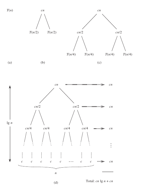
Main observations:
Each level of the tree requires \(cn\) time
There are \(1 + \log_2 n\) levels in total
This gives a total runtime of
\[ T(n) = cn (1 + \log_2 n) = \Theta( n \log n ) \]
Growth of functions
Before moving on, we will briefly discuss asymptotic growth notation
Formally, we are interested in the behaviour of a function \(f(n)\) as \(n \to \infty\)
All functions we consider are from \(\mathbb{N} \to \mathbb{R}\)
Sometimes we may abuse notation and consider functions with domain \(\mathbb{R}\)
\(\Theta\)-notation
- Given a function \(g: \mathbb{N} \to \mathbb{R}\), we define the set
\[\begin{eqnarray*} \Theta(g(n)) = \lbrace f(n)~ &\mid& ~\exists~ c_1, c_2 > 0 \text{ and } N \in \mathbb{N} \text{ such that } \\ && n \geq N \implies 0 \leq c_1 g(n) \leq f(n) \leq c_2 g(n) \rbrace \end{eqnarray*}\]
- That is, \(f(n) \in \Theta(g(n))\) if \(f(n)\) can be asymptotically bounded on both sides by multiples of \(g(n)\)
- We will usually write \(f(n) = \Theta(g(n))\) to mean the same thing.
Note that this definition implicitly requires \(f(n)\) to be asymptotically non-negative
We will assume this here as well as for other asymptotic notations used in this course.
The \(\Theta\) notation is used to indicate exact order of growth
The next two notations indicate upper and lower bounds
\(O\)-notation
- The \(O\)-notation (usually pronounced “big-oh”) indicates an asymptotic upper bound
\[ O(g(n)) = \left\lbrace f(n) ~\mid ~\exists~ c > 0 \text{ and } N \in \mathbb{N} \text{ such that } n \geq N \implies 0 \leq f(n) \leq c g(n) \right\rbrace \]
As before, we usually write \(f(n) = \Theta(g(n))\) to mean \(f(n) \in \Theta(g(n))\)
Note that \(f(n) = \Theta(g(n)) \implies f(n) = O(g(n))\), that is, \(\Theta(g(n)) \subseteq O(g(n))\)
The \(O\)-notation is important because upper bounds are often easier to prove (than lower bounds)
That is often a sufficiently useful characterization of an algorithm
\(\Omega\)-notation
- The \(\Omega\)-notation (pronounced “big-omega”) similarly indicates an asymptotic lower bound
\[ \Omega(g(n)) = \left\lbrace f(n)~ \mid ~\exists~ c > 0 \text{ and } N \in \mathbb{N} \text{ such that } n \geq N \implies 0 \leq c g(n) \leq f(n) \right\rbrace \]
- The proof of the following theorem is an exercise:
\[f(n) = \Theta(g(n)) \iff f(n) = \Omega(g(n)) \text{ and } f(n) = O(g(n))\]
- So, for example, if \(T(n)\) is the running time of insertion sort, then we can say that
\[T(n) = \Omega(n) \text{ and } T(n) = O(n^2)\]
- But not that
\[T(n) = \Theta(n) \text{ or } T(n) = \Theta(n^2)\]
- However, if \(T(n)\) denotes the worst-case running time of insertion sort, then
\[ T(n) = \Theta(n^2) \]
Arithmetic with asymptotic notation
We will often do casual arithmetic with asymptotic notation
Most of the time this is OK, but we should be careful about potential ambiguity
Example: Consider the statement
\[a n^2 + bn + c = an^2 + \Theta(n)\]
Here we use \(\Theta(n)\) to actually mean a function \(f(n) \in \Theta(n)\) (in this case, \(f(n) = bn + c\))
Similarly, we could write
\[2n^2 + \Theta(n) = \Theta(n^2)\]
- This means that whatever the choice of \(f(n) \in \Theta(n)\) in the LHS, \(2n^2 + f(n) = \Theta(n^2)\)
Arithmetic with asymptotic notation
This kind of abuse of notation can sometimes lead to amiguity
For example, if \(f(n) = \Theta(n)\), then
\[ \sum_{i=1}^n f(i) = \Theta(n(n+1)/2) = \Theta(n^2) \]
- We may write the following to mean the same thing:
\[\sum_{i=1}^n \Theta(i)\]
- But this is not the same as \(\Theta(1) + \Theta(2) + \cdots + \Theta(n)\)
- This may not even make sense (what is \(\Theta(2)\) ?)
- Each \(\Theta(i)\) may represent a different function
\(o\)- and \(\omega\)-notation
The \(O\)- and \(\Omega\)-notations indicate bounds that may or may not be asymptotically “tight”
The “little-oh” and “little-omega” notations indicate strictly non-tight bounds
\[ o(g(n)) = \left\lbrace f(n) \colon ~\text{for all}~ c > 0, ~\exists~ N \in \mathbb{N} \text{ such that } n \geq N \implies 0 \leq f(n) \leq c g(n) \right\rbrace \]
- and
\[ \omega(g(n)) = \left\lbrace f(n) \colon ~\text{for all}~ c > 0, ~\exists~ N \in \mathbb{N} \text{ such that } n \geq N \implies 0 \leq c g(n) \leq f(n) \right\rbrace \]
\(o\)- and \(\omega\)-notation
- Essentially, as \(f(n)\) and \(g(n)\) are asymptotically non-negative,
\[f(n) = o(g(n)) \implies \limsup \frac{f(n)}{g(n)} = 0 \implies \lim \frac{f(n)}{g(n)} = 0\]
Similarly, \(f(n) = \omega(g(n)) \implies \lim \frac{f(n)}{g(n)} = \infty\)
Refer to Introduction to Algorithms (Cormen et al) for further properties of asymptotic notation
We will use these properties as and when necessary
Analyzing Divide and Conquer algorithms
As seen for merge sort, the runtime analysis of a divide-and-conquer algorithm usually involves solving a recurrence
Let \(T(n)\) be the running time on a problem of size n
We can write
\[T(n) = \begin{cases} \Theta(1) & \text{if}~ n \leq c \\ a T(n/b) + D(n) + C(n) & \text{otherwise} \end{cases}\]
where \(T(n)\) is constant if the problem is small enough (say \(n \leq c\) for some constant \(c\)), and otherwise
the division step produces \(a\) subproblems, each of size \(n/b\)
\(D(n)\) is the time taken to divide the problem into subproblems,
\(C(n)\) is the time taken to combine the sub-solutions.
Analyzing Divide and Conquer algorithms
There are three common methods to solve recurrences.
The substitution method: guess a bound and then use mathematical induction to prove it correct
The recursion-tree method: convert the recurrence into a tree, and use techniques for bounding summations to solve the recurrence
The master method provides bounds for recurrences of the form \(T(n) = aT(n/b) + f(n)\) for certain functions \(f(n)\) that cover most common cases
The substitution method
The substitution method is basically to
- Guess the form of the solution, and
- Use mathematical induction to verify it
Example (similar to merge sort): Find an upper bound for the recurrence
\[T(n) = 2 T(n/2) + n\]
Suppose we guess that the solution is \(T(n) = O(n \log_2 n)\)
We need to prove that \(T(n) \leq c n \log_2 n\) for some constant \(c > 0\)
Assume this holds for all positive \(m < n\), in particular,
\[ T( n/2 ) \leq \frac{cn}{2} \log_2 \frac{n}{2} \]
The substitution method
- Substituting, we have (provided \(c \geq 1\))
\[\begin{aligned} T(n) & = & 2 T( n/2 ) + n\\ & \leq & 2 \frac12 c n \log_2 (n/2) + n \\ & = & c n \log_2 n - c n \log_2 2 + n \\ & = & c n \log_2 n - c n + n \\ & \leq & c n \log_2 n \\ \end{aligned}\]
The substitution method
Technically, we still need to prove the guess for a boundary condition.
Let’s try for \(n=1\):
- Require \(T(1) \leq c~1 \log_2 1 = 0\)
- Not possible for any realistic value of \(T(1)\)
- So the solution is not true for \(n=1\)
However, for \(n=2\):
- Require \(T(2) \leq c~2 \log_2 2 = 2c\)
- Can be made to hold for some choice of \(c>1\), whatever the value of \(T(2) = 2 T(1) + 2\)
Similarly for \(T(3)\)
Note that for \(n > 3\), the induction step never makes use of \(T(1)\) directly
The substitution method
Remark: be careful not to use asymptotic notation in the induction step
Consider this proof to show \(T(n) = O(n)\), assuming \(T(m) \leq cm\) for \(m<n\)
\[\begin{aligned} T(n) & = & 2 T(n / 2) + n \\ & \leq & 2 c n/2 + n \\ & \leq & cn + n \\ & = & O(n)\end{aligned}\]
The last step is invalid
Unfortunately, making a good guess is not always easy, limiting the usefulness of this method
The recursion tree method
This is the method we used to calculate the merge sort run time
Usually this is helpful to derive a guess that we can then formally prove using recursion
The master method
- The Master theorem: Let \(a \geq 1\) and \(b > 1\) be constants, let \(f(n)\) be a function, and
\[T(n) = a T(n/b) + f(n)\]
- Here \(n/b\) could also floor or ceiling of \(n/b\)
Then \(T(n)\) has the following asymptotic bounds:
If \(f(n) = O(n^{\log_b a - \varepsilon})\) for some constant \(\varepsilon > 0\), then \(T(n) = \Theta(n^{\log_b a})\)
If \(f(n) = \Theta(n^{\log_b a})\), then \(T(n) = \Theta(n^{\log_b a} \log_2 n) = \Theta(f(n) \log_2 n)\)
If \(f(n) = \Omega(n^{\log_b a + \varepsilon})\) for some constant \(\varepsilon > 0\), and if \(a f(n/b) \leq c f(n)\) for some constant \(c < 1\) and all sufficiently large \(n\), then \(T(n) = \Theta(f(n))\)
The master method
We will not prove the master theorem
Note that we are essentially comparing \(f(n)\) with \(n^{\log_b a}\)
whichever is bigger (by a polynomial factor) determines the solution
If they are the same size, we get an additional \(\log n\) factor
Additionally, the third case needs a regularity condition on \(f(n)\)
Exercise: Use the master theorem to obtain the asymptotic order for
\[ T(n) = T(n/2) + cn \]