An Overview of R

# An Overview of R

## Introductory Computer Programming

### Deepayan Sarkar

---

# Software for Statistics

- Computation is an essential part of modern statistics

- Handling large datasets

- Visualization

--
    - Simulation

- Iterative methods

--
- Many softwares are available for such computation, but we will focus on R

---

# Why R?

- Available as [Free](https://en.wikipedia.org/wiki/Free_software_movement) / 
  [Open Source](https://en.wikipedia.org/wiki/The_Open_Source_Definition) Software

- Very popular (both academia and industry)

- Has all essential data analysis tools

- Easy to try out on your own

- Python and Julia are other good alternatives

---

# Outline

- _Interacting_ with R

- Installing and running R

- Basics of using R

- Some examples

---

# Interacting with R

* R is most commonly used as a [REPL](https://en.wikipedia.org/wiki/Read-eval-print_loop) (Read-Eval-Print-Loop)

* When it is started, R waits for user input

* User inputs expression

* R evaluates and prints result

* Waits for more input

* Several _interfaces_ are available to help in this process

* Recommended interface: [_RStudio_](https://posit.co/products/open-source/rstudio/)

* Julia and Python have the same REPL interface

* Another popular interface: [_Jupyter_](https://jupyter.org/) (Julia, Python, R)

---

# Installing R and RStudio

* Go to <https://cran.icts.res.in/> (or choose a [mirror](https://cran.r-project.org/mirrors.html) first)

* Follow instructions depending on your platform (Windows for most of you)
--

* For RStudio, go to <https://posit.co/download/rstudio-desktop/>

---

# Running R

* Once installed, you can start RStudio (or R directly) to get something like this:

```
R version 4.3.1 (2023-06-16) -- "Beagle Scouts"
Copyright (C) 2023 The R Foundation for Statistical Computing
Platform: x86_64-apple-darwin20 (64-bit)

R is free software and comes with ABSOLUTELY NO WARRANTY.
You are welcome to redistribute it under certain conditions.
Type 'license()' or 'licence()' for distribution details.

Natural language support but running in an English locale

R is a collaborative project with many contributors.
Type 'contributors()' for more information and
'citation()' on how to cite R or R packages in publications.

Type 'demo()' for some demos, 'help()' for on-line help, or
'help.start()' for an HTML browser interface to help.
Type 'q()' to quit R.

> 
```

* The `>` represents a _prompt_ indicating that R is waiting for input.

* The difficult part is to learn what to do next

---

# The R REPL essentially works like a calculator

```r
34 * 23 + 10
```

```
[1] 792
```

```r
27 + 1 / 7
```

```
[1] 27.14286
```

```r
2^10
```

```
[1] 1024
```
--

```r
exp(2)
```

```
[1] 7.389056
```

---

# The Python REPL is very similar

```python
34 * 23 + 10
```

```
792
```

```python
27 + 1 / 7
```

```
27.142857142857142
```

---

# But not exactly the same

```python
2^10
```

```
8
```

```python
2 ** 10
```

```
1024
```

* The _power_ operator is different in R and Python

* `a^b` means something different in Python (any guesses?)

---

# But not exactly the same

```python
exp(2)
```

```
Traceback (most recent call last):
  File "<stdin>", line 1, in <module>
NameError: name 'exp' is not defined
```

* Results in error message

* Essentially says that the `exp()` function is not defined

---

# NumPy for scientific computing in Python

* `exp()` is defined in an _optional_ package (_NumPy_) in Python

```python
from numpy import *
exp(2)
```

```
7.38905609893065
```

```python
sin(pi / 6)
```

```
0.49999999999999994
```

* Compare with R

```r
exp(2)
```

```
[1] 7.389056
```

```r
sin(pi / 6)
```

```
[1] 0.5
```

---

# R supports mathematical functions

---

```r
sqrt(5 * 125)
```

```
[1] 25
```

```r
log(120)
```

```
[1] 4.787492
```

```r
factorial(10)
```

```
[1] 3628800
```

```r
log(factorial(10))
```

```
[1] 15.10441
```

---

```r
choose(15, 5)
```

```
[1] 3003
```

```r
factorial(15) / (factorial(10) * factorial(5))
```

```
[1] 3003
```

```r
choose(1500, 2)
```

```
[1] 1124250
```

```r
factorial(1500) / (factorial(1498) * factorial(2))
```

```
[1] NaN
```

* Why does this fail?

* Numerical results do not always match theory!

---

# Variables and Functions

* All examples so far use explicit values (like a calculator)

* But R is much more: it is a full programming language

* Two basic features: variables and functions

---

# R supports variables

```r
x <- 2     # assignment can be done using <-
y = 10     # it can also be done using = 
x^y
```

```
[1] 1024
```

```r
y^x
```

```
[1] 100
```

```r
factorial(y)
```

```
[1] 3628800
```

```r
log(factorial(y), base = x) # = also used to specify arguments
```

```
[1] 21.79106
```

---

# R has functions

* Most operations are performed using functions

* We have already seen several examples (`choose`, `log`)

* A function is usually called by name, followed by arguments in
  parentheses

```r
choose(y, x)
```

```
[1] 45
```

```r
log(y)
```

```
[1] 2.302585
```
  
---

# R has functions and operators

* Many operations are done using _operators_

```r
x + y
```

```
[1] 12
```

```r
x * y
```

```
[1] 20
```

* These are actually also functions

```r
`+`(x, y)
```

```
[1] 12
```

```r
`*`(x, y)
```

```
[1] 20
```

---

# Function arguments

---

* Functions have named input arguments

* Easy to identify using the `str()` function

```r
str(choose)
```

```
function (n, k)  
```

* When calling the function, arguments are identified by position

```r
choose(y, x) # n = y, k = x
```

```
[1] 45
```

---

* Some arguments can have default values

```r
str(log)
```

```
function (x, base = exp(1))  
```

* These arguments are optional, but can be specified if necessary

```r
log(y)
```

```
[1] 2.302585
```

```r
log(y, 2)
```

```
[1] 3.321928
```

---

* Arguments can also be specified by name

```r
choose(n = y, k = x)
```

```
[1] 45
```

```r
log(y, base = x)
```

```
[1] 3.321928
```

---

* Names override matching by position

```r
choose(k = x, n = y)
```

```
[1] 45
```

```r
log(base = x, y)
```

```
[1] 3.321928
```

* Common practice is to use a mix of both

---

# Vectors and vectorization

* All calculations so far have been with ‘scalar’ numbers

* Statistical computations are usually with a _collection_ of numbers

* Example: sample mean, sample median, ...

* The data structure we use for this is called a _vector_

* Also sometimes called _arrays_ in other programming languages

---

# A simple ways to generate vectors

* The `seq()` function or the `:` operator

```r
x:y
```

```
[1]  2  3  4  5  6  7  8  9 10
```

```r
seq(x, y)
```

```
[1]  2  3  4  5  6  7  8  9 10
```

* `seq()` has more options

```r
seq(x, y, by = 0.1)
```

```
 [1]  2.0  2.1  2.2  2.3  2.4  2.5  2.6  2.7  2.8  2.9  3.0  3.1  3.2  3.3  3.4  3.5  3.6  3.7  3.8
[20]  3.9  4.0  4.1  4.2  4.3  4.4  4.5  4.6  4.7  4.8  4.9  5.0  5.1  5.2  5.3  5.4  5.5  5.6  5.7
[39]  5.8  5.9  6.0  6.1  6.2  6.3  6.4  6.5  6.6  6.7  6.8  6.9  7.0  7.1  7.2  7.3  7.4  7.5  7.6
[58]  7.7  7.8  7.9  8.0  8.1  8.2  8.3  8.4  8.5  8.6  8.7  8.8  8.9  9.0  9.1  9.2  9.3  9.4  9.5
[77]  9.6  9.7  9.8  9.9 10.0
```

???

---

# Another simple ways to generate vectors: simulation

---

* Real data will usually need to be imported from some external source (later)

* Easy way to generate fake data: use a random number generator

* Example: `sample()` takes SRSWR / SRSWOR from a population

```r
sample(1:20)
```

```
 [1] 16 19  7 18 12  3 20  9 14  6  5  2 15 17  8 13 10  4 11  1
```

```r
sample(1:10, 5)
```

```
[1]  3  9  1  5 10
```

---

* Default choice is to take SRS without replacement

```r
sample(1:10, 20)
```

```
Error in sample.int(length(x), size, replace, prob): cannot take a sample larger than the population when 'replace = FALSE'
```

```r
str(sample)                        # check argument names
```

```
function (x, size, replace = FALSE, prob = NULL)  
```

```r
sample(1:10, 20, replace = TRUE)   # SRSWR
```

```
 [1]  5 10  2  4  8  6  1  6  1  5  2 10  7  6  6  7  1  2  5  4
```

---

* More common to simulate from standard distributions

```r
runif(20)                      # Uniform(0, 1)
```

```
 [1] 0.3053615 0.1527969 0.9544736 0.1275601 0.7926520 0.3559776 0.3746061 0.6588806 0.8453407
[10] 0.4561515 0.8768534 0.7270854 0.8098272 0.4169682 0.5745668 0.7501082 0.4118677 0.9503846
[19] 0.3066031 0.7305853
```

```r
rnorm(20)                      # Normal(0, 1)
```

```
 [1]  0.89115326 -0.81426555  1.13429632  0.04684551 -1.11403664  0.29115863  1.07548368 -0.27692420
 [9] -0.53045524  0.18933636  0.09635957  0.81507845 -1.67489130  0.65240454 -0.67079568 -1.28006272
[17] -1.30565431 -1.01201508 -0.86093174  0.52684660
```

```r
rnorm(20, mean = 1, sd = 2)    # Normal(1, 4)
```

```
 [1]  1.2954811  4.7298128 -1.7857474  2.2258012 -1.9979038  0.4525213  4.1736062  1.2825705
 [9]  1.6074737  0.8810607 -0.4162386  2.2950240  2.2957853 -1.0800112  2.7910280  2.3283533
[17]  2.2274600 -0.0746961  1.0713221 -0.3204942
```

---

# What can we do with vectors?

* To do anything, we usually first assign it to a variable

```r
x <- rnorm(50)
```

* We can _print_ the vector (by just typing its name)

```r
x
```

```
 [1] -2.227478187  2.094353947 -0.033814973 -0.220856292 -1.149963524  0.408173501 -0.411488837
 [8] -1.063422582 -1.701321281 -0.097193951  0.786428966  0.604681731 -0.236270674 -0.536386876
[15] -1.362862694  1.360117333 -0.144368264 -1.356851185  0.924968261  0.343918354 -1.209425269
[22]  0.366876257  0.139233387 -1.502580980  0.176345435 -1.696108677  0.472131982  1.159065918
[29] -1.401299453  0.476863691  0.509902009 -1.576790283 -0.644674505 -1.406436226 -0.391760755
[36] -0.405671655 -1.990810546  0.575063842 -0.104819770  1.506343340 -0.403221260  0.005669989
[43] -0.401022628  0.867013297  0.510874538 -1.833891317  2.017811867 -0.005421944  1.424590998
[50] -0.791741513
```

---

# Summary functions

* We can call _summary_ functions that compute various statistics

```r
sum(x)
```

```
[1] -9.577527
```

```r
length(x)
```

```
[1] 50
```

```r
sum(x) / length(x)
```

```
[1] -0.1915505
```

```r
mean(x)
```

```
[1] -0.1915505
```

---

# Vectorized functions

---

* Some functions operate on vectors _elementwise_

* In fact, most standard mathematical functions and operators are
  _vectorized_

???

To illustrate this, suppose we want to compute all the binomial
coefficients and choose R with n equal to 15. R in this case, we’ll
take the values 0, 1, 2, etc, all the way up to 15. It’s a good habit
to use variables instead of constants when writing code so that the
same code can be reused later for different inputs. Let’s define a
variable to represent the value of n equal to 15. We’ll just call it
n. The next thing we need is to create a vector containing all the
values of R that we want. As we saw, we can use the colon operator to
create the vector from 1-15, but of course this is missing 0. Let me
use 0-15. In fact, let’s use the variable that we have just
defined. That will give us the vector 0-15. Let’s store this in a
variable so that we can use it later. We are now ready to compute n
choose R. Let’s verify that this is our n, 15, R is the vector with
values 0-15. Then instead of doing a for loop or anything like that, I
will just call choose n, R. This call looks exactly similar to what we
have done earlier. Just as we computed 15 choose 5, we are now
computing n choose R. It just happens that one of the inputs in this
function is a vector. That result is also a vector. Actually, both of
these could be vectors, but that’s not very useful for us right
now. In the next video, we will combine many of the things we have
learned so far to study the binomial distribution or at least some
simple properties of it.

---

* Example: Binomial coefficients

```r
N <- 15
x <- seq(0, N)
```

```r
N
```

```
[1] 15
```

```r
x
```

```
 [1]  0  1  2  3  4  5  6  7  8  9 10 11 12 13 14 15
```

```r
choose(N, x)
```

```
 [1]    1   15  105  455 1365 3003 5005 6435 6435 5005 3003 1365  455  105   15    1
```

---

* Example: Binomial probabilities

$$
P(X = x) = { n \choose x } p^x (1-p)^{n-x}
$$

* Using formula directly

```r
N <- 15
x <- seq(0, N)
p <- 0.25
choose(N, x) * p^x * (1-p)^(N-x)
```

```
 [1] 1.336346e-02 6.681731e-02 1.559070e-01 2.251991e-01 2.251991e-01 1.651460e-01 9.174777e-02
 [8] 3.932047e-02 1.310682e-02 3.398065e-03 6.796131e-04 1.029717e-04 1.144130e-05 8.800998e-07
[15] 4.190952e-08 9.313226e-10
```

---

* Example: Binomial probabilities

$$
P(X = x) = { n \choose x } p^x (1-p)^{n-x}
$$

* Using specialized built-in `dbinom()` function

```r
N <- 15
x <- seq(0, N)
p <- 0.25
dbinom(x, size = N, prob = p)
```

---

# Computing probability of events

---

* Example: probability that $X$ is even

```r
seq(0, N, by = 2)
```

```
[1]  0  2  4  6  8 10 12 14
```

```r
sum(dbinom(seq(0, N, by = 2), size = N, prob = p))
```

```
[1] 0.5000153
```

---

* Example: probability that $X \leq 7$

```r
sum(dbinom(0:7, size = N, prob = p))
```

```
[1] 0.9827002
```

* This is actually just the CDF, which can be calculated using `pbinom()`

```r
pbinom(7, size = N, prob = p)
```

```
[1] 0.9827002
```

---

# Computing expectation

```r
p.x <- dbinom(x, size = N, prob = p)
p.x
```

```r
x * p.x
```

```
 [1] 0.000000e+00 6.681731e-02 3.118141e-01 6.755972e-01 9.007963e-01 8.257299e-01 5.504866e-01
 [8] 2.752433e-01 1.048546e-01 3.058259e-02 6.796131e-03 1.132688e-03 1.372956e-04 1.144130e-05
[15] 5.867332e-07 1.396984e-08
```

```r
sum(x * p.x)  # expectation from definition
```

```
[1] 3.75
```

```r
N * p         # same answer in this case
```

```
[1] 3.75
```

---

# R can draw graphs

```r
plot(x, p.x, ylab = "Probability", pch = 16)
title(main = sprintf("Binomial(%g, %g)", N, p))
abline(h = 0, col = "grey")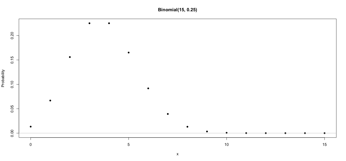
```

![plot of chunk unnamed-chunk-44](figures/roverview-1-unnamed-chunk-44-1.png)

---

# A more complicated example: Law of Large Numbers

---

* Simulate 100 coin tosses with $P(\text{head}) = p$

```r
p <- 0.25
z <- rbinom(100, size = 1, prob = p)
z
```

```
  [1] 0 1 0 0 0 0 0 0 0 0 0 0 0 0 1 0 0 0 0 1 0 1 1 0 1 1 0 0 0 1 0 0 1 0 0 0 0 0 0 0 1 0 0 0 0 0 0
 [48] 0 0 0 0 0 1 1 0 0 1 0 1 0 0 1 0 0 0 0 1 0 0 0 0 1 0 0 0 0 0 0 0 0 1 0 0 0 0 0 0 0 0 1 0 1 0 0
 [95] 1 1 1 0 0 0
```

* We know sample proportion should ‘converge’ to $p$

* Does simulated data show this behaviour?

---

* Useful function: `cumsum()` (cumulative sum)

```r
cumsum(z)
```

```
  [1]  0  1  1  1  1  1  1  1  1  1  1  1  1  1  2  2  2  2  2  3  3  4  5  5  6  7  7  7  7  8  8
 [32]  8  9  9  9  9  9  9  9  9 10 10 10 10 10 10 10 10 10 10 10 10 11 12 12 12 13 13 14 14 14 15
 [63] 15 15 15 15 16 16 16 16 16 17 17 17 17 17 17 17 17 17 18 18 18 18 18 18 18 18 18 19 19 20 20
 [94] 20 21 22 23 23 23 23
```

* Cumulative mean can be computed by elementwise division

```r
cumsum(z) / 1:100
```

```
  [1] 0.00000000 0.50000000 0.33333333 0.25000000 0.20000000 0.16666667 0.14285714 0.12500000
  [9] 0.11111111 0.10000000 0.09090909 0.08333333 0.07692308 0.07142857 0.13333333 0.12500000
 [17] 0.11764706 0.11111111 0.10526316 0.15000000 0.14285714 0.18181818 0.21739130 0.20833333
 [25] 0.24000000 0.26923077 0.25925926 0.25000000 0.24137931 0.26666667 0.25806452 0.25000000
 [33] 0.27272727 0.26470588 0.25714286 0.25000000 0.24324324 0.23684211 0.23076923 0.22500000
 [41] 0.24390244 0.23809524 0.23255814 0.22727273 0.22222222 0.21739130 0.21276596 0.20833333
 [49] 0.20408163 0.20000000 0.19607843 0.19230769 0.20754717 0.22222222 0.21818182 0.21428571
 [57] 0.22807018 0.22413793 0.23728814 0.23333333 0.22950820 0.24193548 0.23809524 0.23437500
 [65] 0.23076923 0.22727273 0.23880597 0.23529412 0.23188406 0.22857143 0.22535211 0.23611111
 [73] 0.23287671 0.22972973 0.22666667 0.22368421 0.22077922 0.21794872 0.21518987 0.21250000
 [81] 0.22222222 0.21951220 0.21686747 0.21428571 0.21176471 0.20930233 0.20689655 0.20454545
 [89] 0.20224719 0.21111111 0.20879121 0.21739130 0.21505376 0.21276596 0.22105263 0.22916667
 [97] 0.23711340 0.23469388 0.23232323 0.23000000
```

---

```r
plot(1:100, type = "n", ylim = c(0, 1), ylab = "Sample proportion")
for (i in 1:50) {                                 # Repeat multiple times and plot
    z <- rbinom(100, size = 1, prob = p)
    lines(1:100, cumsum(z) / 1:100, col = sample(colors(), 1))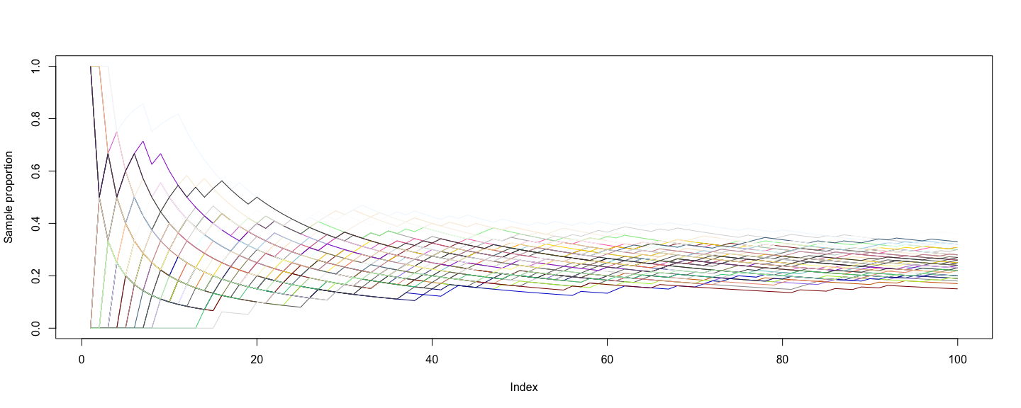
}
```

![plot of chunk unnamed-chunk-48](figures/roverview-1-unnamed-chunk-48-1.png)

---

# Summary: R is a full programming language

* Variables

* Functions

* Control flow structures

* Distinguishing feature: Focus on _vectors_ and _vectorized operations_

* We will next learn the language more formally