Static R Graphics: A Brief Introduction
Deepayan Sarkar
Grid graphics, lattice and ggplot2
These represent two very different philosophical approaches to graphics
lattice is in many ways a natural successor to traditional graphics
ggplot2 represents a completely different declarative approach
An example: Anscombe’s quartet
I will try to illustrate this with an example
Anscombe (1973) introduced four artificial bivariate datasets to emphasize the importance of graphics
The datasets all had the same means, standard deviations, and correlation
'data.frame':   11 obs. of  8 variables:
 $ x1: num  10 8 13 9 11 14 6 4 12 7 ...
 $ x2: num  10 8 13 9 11 14 6 4 12 7 ...
 $ x3: num  10 8 13 9 11 14 6 4 12 7 ...
 $ x4: num  8 8 8 8 8 8 8 19 8 8 ...
 $ y1: num  8.04 6.95 7.58 8.81 8.33 ...
 $ y2: num  9.14 8.14 8.74 8.77 9.26 8.1 6.13 3.1 9.13 7.26 ...
 $ y3: num  7.46 6.77 12.74 7.11 7.81 ...
 $ y4: num  6.58 5.76 7.71 8.84 8.47 7.04 5.25 12.5 5.56 7.91 ...
An example: Anscombe’s quartet
      x1       x2       x3       x4       y1       y2       y3       y4
9.000000 9.000000 9.000000 9.000000 7.500909 7.500909 7.500000 7.500909
      x1       x2       x3       x4       y1       y2       y3       y4
3.316625 3.316625 3.316625 3.316625 2.031568 2.031657 2.030424 2.030579
[1] 0.8164205 0.8162365 0.8162867 0.8165214
- How can we plot all four datasets together?
Anscombe’s quartet using traditional graphics
Traditional graphics thinks of this as four different data sets
The function to create scatter plots is plot()
Multiple plots can be put in the same figure using par(mfrow = ...)
Several ways of specifying variable names inside dataset:
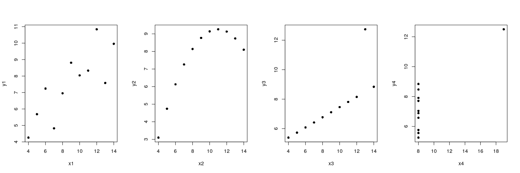
Anscombe’s quartet using traditional graphics
![plot of chunk unnamed-chunk-3]()
Anscombe’s quartet using traditional graphics
xrng <- with(anscombe, range(x1, x2, x3, x4))
yrng <- with(anscombe, range(y1, y2, y3, y4))   ## common axis limits
par(mfrow = c(1, 4))
plot(y1 ~ x1, data = anscombe, pch = 16, xlim = xrng, ylim = yrng)
plot(y2 ~ x2, data = anscombe, pch = 16, xlim = xrng, ylim = yrng)
plot(y3 ~ x3, data = anscombe, pch = 16, xlim = xrng, ylim = yrng)
plot(y4 ~ x4, data = anscombe, pch = 16, xlim = xrng, ylim = yrng)
![plot of chunk unnamed-chunk-4]()
Anscombe’s quartet using lattice and ggplot2
anscombe.long <-
    with(anscombe, data.frame(x = c(x1, x2, x3, x4),
                              y = c(y1, y2, y3, y4),
                              which = rep(c("1", "2", "3", "4"), each = 11)))
str(anscombe.long)
'data.frame':   44 obs. of  3 variables:
 $ x    : num  10 8 13 9 11 14 6 4 12 7 ...
 $ y    : num  8.04 6.95 7.58 8.81 8.33 ...
 $ which: Factor w/ 4 levels "1","2","3","4": 1 1 1 1 1 1 1 1 1 1 ...
Anscombe’s quartet using lattice
![plot of chunk unnamed-chunk-6]()
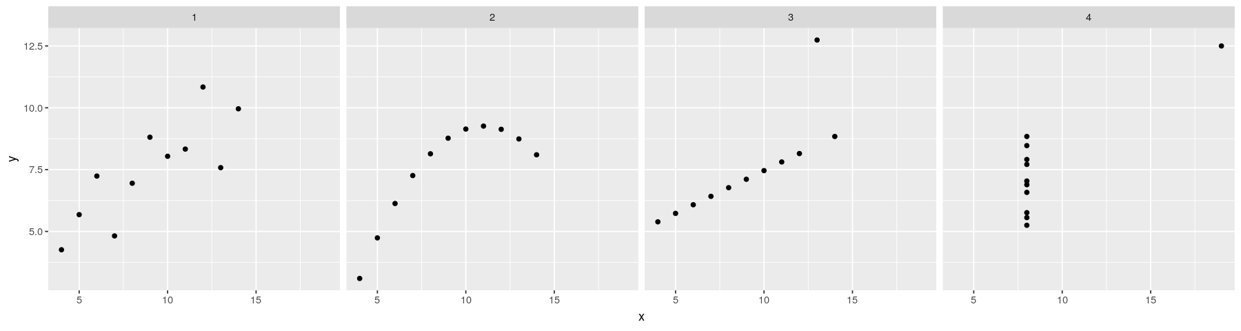
Anscombe’s quartet using ggplot2
![plot of chunk unnamed-chunk-7]()
Anscombe’s quartet using lattice and ggplot2
The approaches share many common features
Both Capable of plotting subsets of data (indexed by categorical variables)
- This idea is known by several names: small multiples, conditioning, facetting
Both makes efficient use of available space (common scales, common axes)
Different visual appearance, but that is superficial (different default themes)
Anscombe’s quartet using lattice and ggplot2
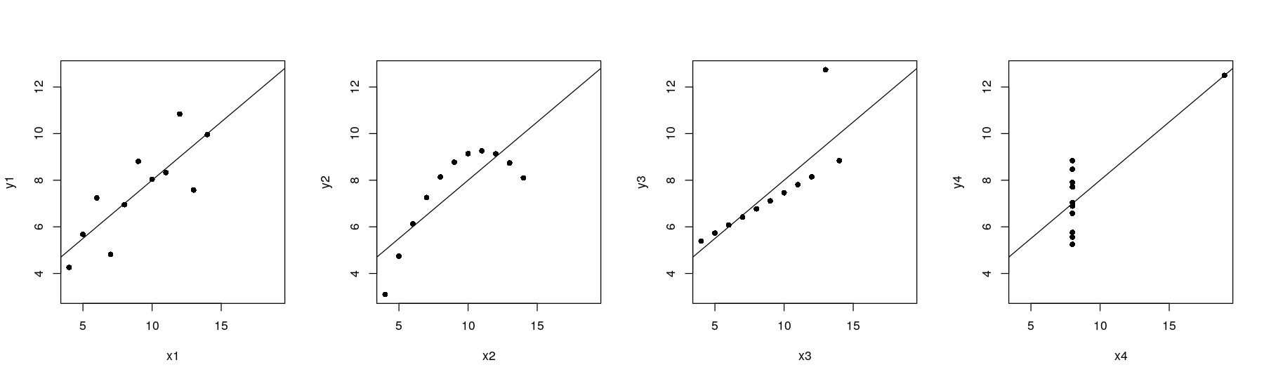
Anscombe’s quartet with regression lines
xrng <- with(anscombe, range(x1, x2, x3, x4))
yrng <- with(anscombe, range(y1, y2, y3, y4))
par(mfrow = c(1, 4))
plot(y1 ~ x1, anscombe, pch = 16, xlim = xrng, ylim = yrng)
abline(lm(y1 ~ x1, anscombe))  ## lm() fits regression line, abline() adds the line to current plot
plot(y2 ~ x2, anscombe, pch = 16, xlim = xrng, ylim = yrng)
abline(lm(y2 ~ x2, anscombe))
plot(y3 ~ x3, anscombe, pch = 16, xlim = xrng, ylim = yrng)
abline(lm(y3 ~ x3, anscombe))
plot(y4 ~ x4, anscombe, pch = 16, xlim = xrng, ylim = yrng)
abline(lm(y4 ~ x4, anscombe))
![plot of chunk unnamed-chunk-8]()
Anscombe’s quartet with regression lines
The traditional graphics approach is to add the line after the plot is drawn
In general, a plot is never finished, you can always add more points, lines, text, …
This is possible because there is only one plot !
lattice and ggplot2 need alternative solutions
The ggplot2 solution is to allow plots to have multiple layers
The lattice solution is to allow user to fully specify the procedure used to display data
Regression lines: the ggplot2 solution
![plot of chunk unnamed-chunk-9]()
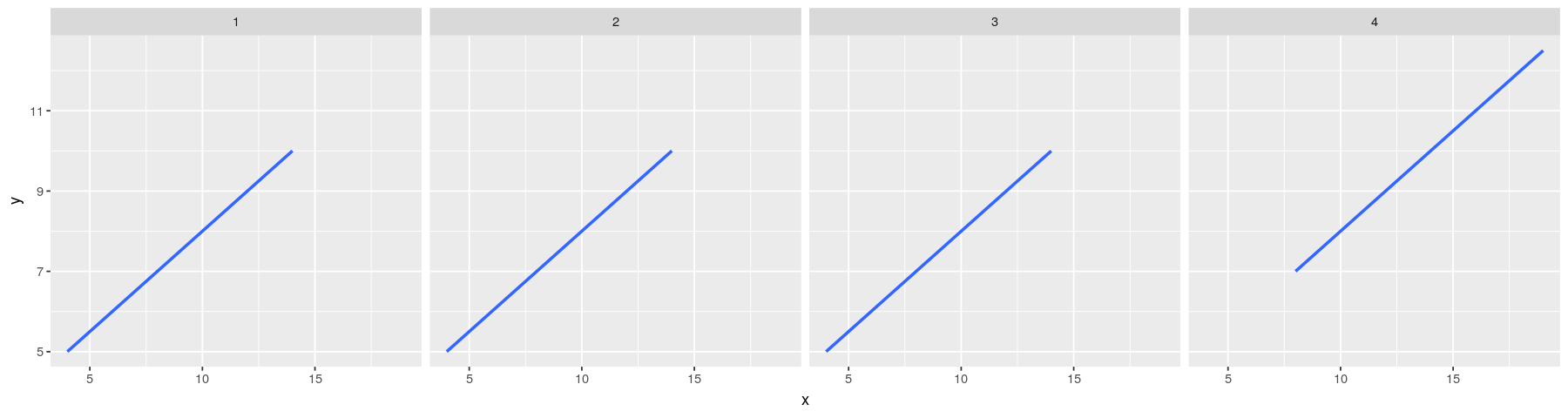
Regression lines: the ggplot2 solution
- Plot with regression line only
![plot of chunk unnamed-chunk-10]()
Regression lines: the ggplot2 solution
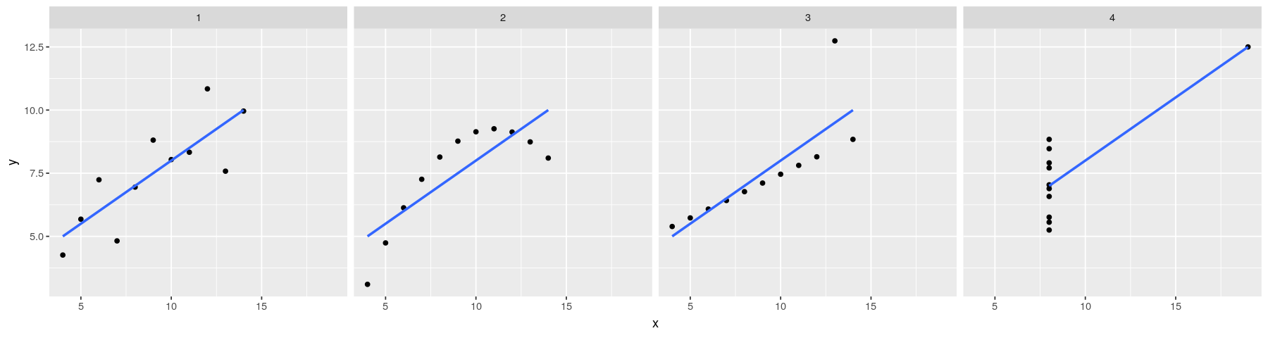
- Plot with both points and regression lines
![plot of chunk unnamed-chunk-11]()
Regression lines: the lattice solution
The lattice solution is actually very similar to the traditional graphics solution
Basically, we want to do the following for each data subset x, y:
For lattice, we need to encapsulate this procedure into a function
- This function is then supplied to the
xyplot() function as the panel argument
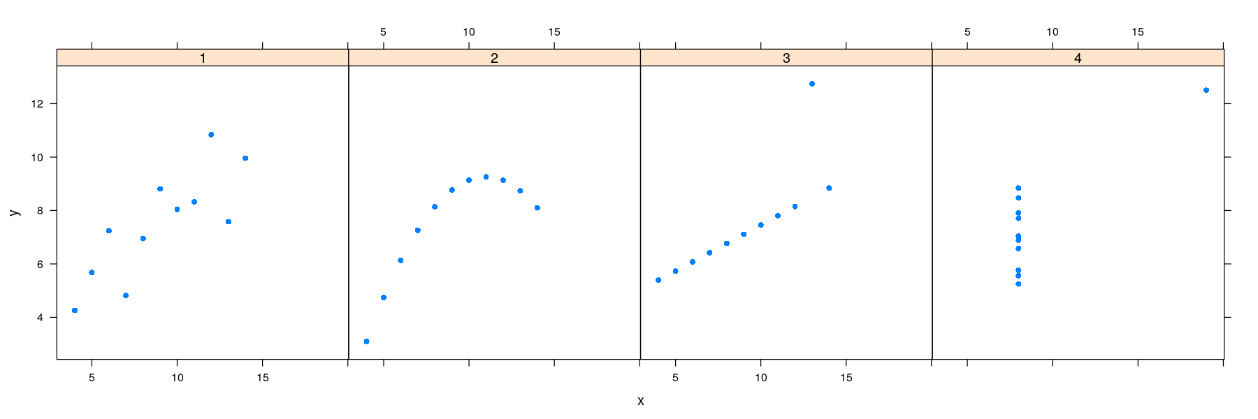
Regression lines: the lattice solution
![plot of chunk unnamed-chunk-13]()
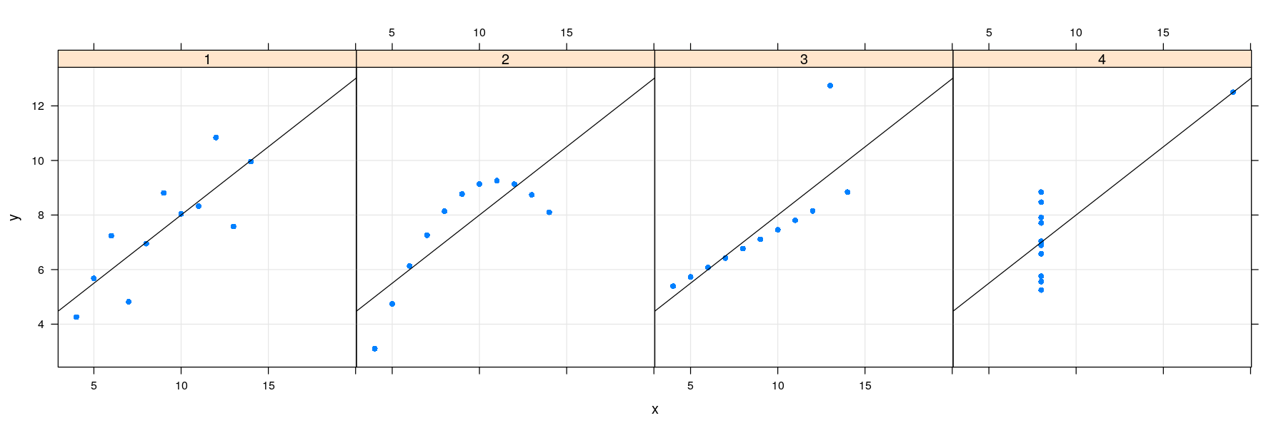
Regression lines: the lattice solution
- Plot with grid, points, and regression line
![plot of chunk unnamed-chunk-14]()
Regression lines: the lattice solution
- lattice also supports a layering mechanism similar to ggplot2
![plot of chunk unnamed-chunk-15]()
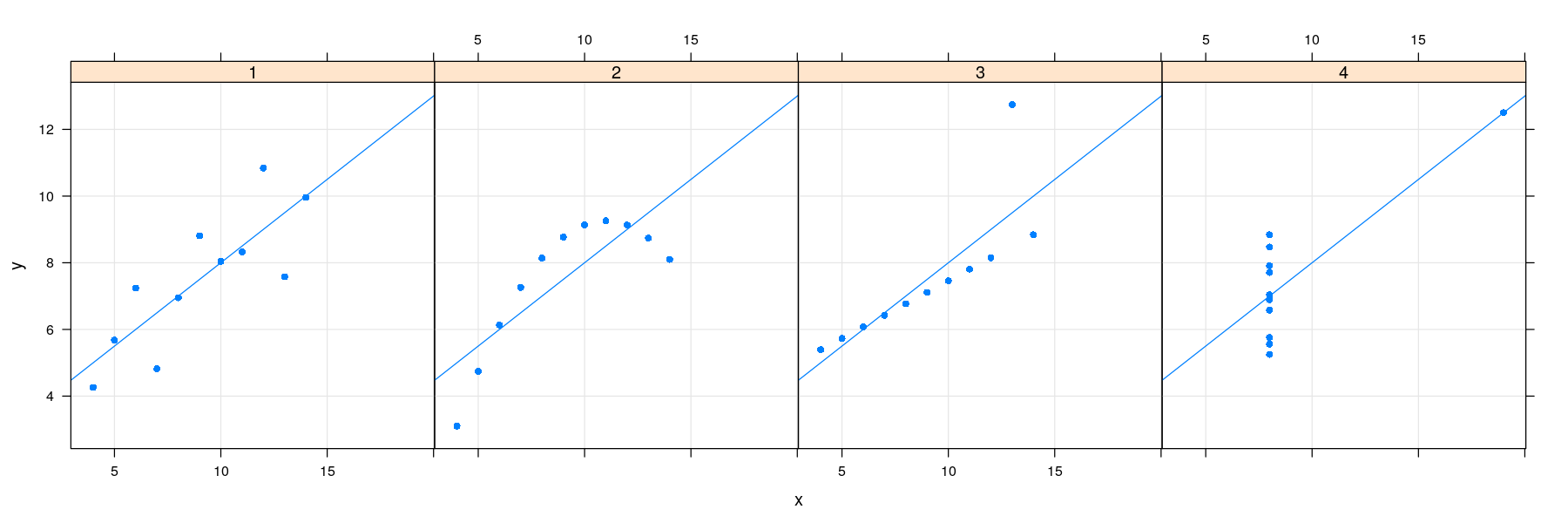
Regression lines: the lattice solution
- Common customizations like these are also supported directly through optional arguments
![plot of chunk unnamed-chunk-16]()
Brief history of R graphics
R is an Open Source / Free Software re-implementation / dialect of S
The original implementation, available commercially as S-PLUS, was developed at Bell Labs
Both traditional graphics and Trellis graphics were part of the original S
Remembering this helps in understanding the design of graphics in R
Origins of the graphics model
The abstract graphics model in S may be described as a “painter’s model”:
a graphic is built out of a small set of primitives such as line segments, polygons, text, etc., and
later elements are drawn on top of earlier ones
no provision for deleting an element once it was drawn
except to start a completely new graphic
Advantage: both input and output could be abstracted
Graphics functions called by users would internally call these primitives
For output, the primitives could be implemented differently depending on the target “device”
This leads to a concept of graphics devices
Postscript or PDF files for printing,
Hardware devices such as pen plotters,
On-screen devices for interactive viewing (different for Windows / Linux / Mac)
Image files (JPG / PNG) for inclusion in a web page
Device-specific implementations of the primitives are known as device drivers
New drivers can be written to support new kinds of output formats
See ?Devices for more details.
This is how R has solved the problem of cross-platform consistency for graphics
The drawback is that more advanced / interactive features are not available
Traditional graphics
The core of the traditional R graphics system is the suite of functions available in the graphics package,
Various add-on packages providing further functionality.
The full list of functions can be seen using
Commonly used high-level traditional graphics functions
plot() |
Scatter Plot, Time-series Plot (with type="l") |
boxplot() |
Comparative Box-and-Whisker Plots |
barplot() |
Bar Plot |
dotchart() |
Cleveland Dot Plot |
hist() |
Histogram |
plot(density()) |
Kernel Density Plot |
qqnorm() |
Normal Quantile-Quantile Plot |
qqplot() |
Two-sample Quantile-Quantile Plot |
stripchart() |
Stripchart (Comparative 1-D Scatter Plots) |
pairs() |
Scatter-Plot Matrix |
lattice defines analogous functions with different names
xyplot() |
Scatter Plot, Time-series Plot (with type="l") |
bwplot() |
Comparative Box-and-Whisker Plots |
barchart() |
Bar Plot |
dotplot() |
Cleveland Dot Plot |
histogram() |
Histogram |
densityplot() |
Kernel Density Plot |
qqmath() |
Normal Quantile-Quantile Plot |
qq() |
Two-sample Quantile-Quantile Plot |
stripplot() |
Stripchart (Comparative 1-D Scatter Plots) |
splom() |
Scatter-Plot Matrix |
Grammar of graphics: Main components
Aesthetic mappings that map data values to some aspect in the displayed graph, such as
- coordinate positions
- color, shape, size
- group, …
geometric types used to render the mapped data, e.g.,
- points, lines, polygons
- more complex types such as a box-and-whisker plot
statistical transformations that are applied to the data beforehand, such as
- binning for histograms
- computation of kernel density estimates.
Scales that give a visual indication of the aesthetic mappings, e.g.,
- axis annotation for position mapping
- legends for mapping to color, size, etc.
Faceting (conditioning) to produce small multiples
Grammar of graphics - built-in geoms and stats
 [1] "geom_abline"     "geom_area"       "geom_bar"        "geom_bin2d"      "geom_blank"      "geom_boxplot"
 [7] "geom_col"        "geom_contour"    "geom_count"      "geom_crossbar"   "geom_curve"      "geom_density"
[13] "geom_density_2d" "geom_density2d"  "geom_dotplot"    "geom_errorbar"   "geom_errorbarh"  "geom_freqpoly"
[19] "geom_hex"        "geom_histogram"  "geom_hline"      "geom_jitter"     "geom_label"      "geom_line"
[25] "geom_linerange"  "geom_map"        "geom_path"       "geom_point"      "geom_pointrange" "geom_polygon"
[31] "geom_qq"         "geom_qq_line"    "geom_quantile"   "geom_raster"     "geom_rect"       "geom_ribbon"
[37] "geom_rug"        "geom_segment"    "geom_sf"         "geom_sf_label"   "geom_sf_text"    "geom_smooth"
[43] "geom_spoke"      "geom_step"       "geom_text"       "geom_tile"       "geom_violin"     "geom_vline"
 [1] "stat_bin"            "stat_bin_2d"         "stat_bin_hex"        "stat_bin2d"          "stat_binhex"
 [6] "stat_boxplot"        "stat_contour"        "stat_count"          "stat_density"        "stat_density_2d"
[11] "stat_density2d"      "stat_ecdf"           "stat_ellipse"        "stat_function"       "stat_identity"
[16] "stat_qq"             "stat_qq_line"        "stat_quantile"       "stat_sf"             "stat_sf_coordinates"
[21] "stat_smooth"         "stat_spoke"          "stat_sum"            "stat_summary"        "stat_summary_2d"
[26] "stat_summary_bin"    "stat_summary_hex"    "stat_summary2d"      "stat_unique"         "stat_ydensity"
References
Anscombe, Francis J. 1973. “Graphs in Statistical Analysis.” The American Statistician 27 (1). Taylor & Francis Group: 17–21.