Collinearity: Impact and Possible Remedies
Deepayan Sarkar
What is collinearity?
Exact dependence between columns of \(\mathbf{X}\) make coefficients non-estimable
Collinearity refers to the situation where some columns are almost dependent
Why is this a problem?
Individual coefficient estimates \(\hat{\beta}_j\) become unstable (high variance)
Standard errors are large, tests have low power
On the other hand, \(\hat{\mathbf{y}} = \mathbf{H} \mathbf{y}\) is not particularly affected
Detecting collinearity
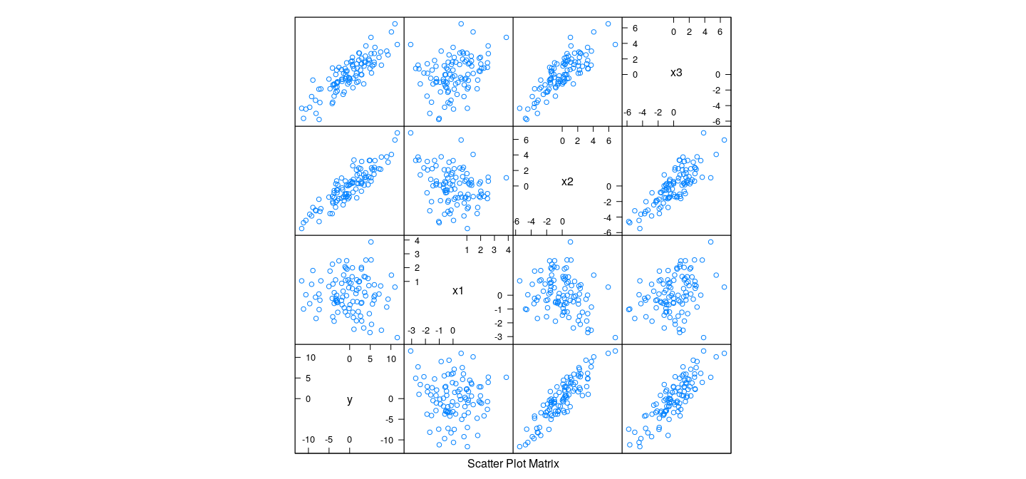
Collinearity in pairs of variables are easily seen in scatter plots
However, higher dimensional collinearity may not be readily apparent
Example:
n <- 100
z1 <- rnorm(n)
z2 <- rnorm(n)
x1 <- z1 + z2 + 0.1 * rnorm(n)
x2 <- z1 - 2 * z2 + 0.1 * rnorm(n)
x3 <- 2 * z1 - z2 + 0.1 * rnorm(n)
y <- x1 + 2 * x2 + 2 * rnorm(n) # x3 has coefficient 0
d3 <- data.frame(y, x1, x2, x3)
cor(d3)
y x1 x2 x3
y 1.00000000 -0.05350867 0.8930301 0.8498399
x1 -0.05350867 1.00000000 -0.2750082 0.3047524
x2 0.89303013 -0.27500823 1.0000000 0.8287638
x3 0.84983991 0.30475236 0.8287638 1.0000000Detecting collinearity
Detecting collinearity
- In this case, a 3-D plot is sufficient (but not enough for higher-dimensional collinearity)
Detecting collinearity
Pairwise scatter plots do not indicate unusual dependence
However, each \(X_{* j}\) is highly dependent on others
[1] 0.9816998[1] 0.9936826[1] 0.9938004Impact of collinearity
- This results in increased uncertainty in coefficient estimates
Call:
lm(formula = y ~ x1 + x2 + x3, data = d3)

Residuals:
    Min      1Q  Median      3Q     Max
-4.5620 -1.3326 -0.0007  1.6717  4.5924

Coefficients:
            Estimate Std. Error t value Pr(>|t|)
(Intercept)  0.04719    0.20629   0.229   0.8195
x1           1.09743    1.12399   0.976   0.3313
x2           2.38916    1.12119   2.131   0.0357 *
x3          -0.33411    1.12900  -0.296   0.7679
---
Signif. codes:  0 '***' 0.001 '**' 0.01 '*' 0.05 '.' 0.1 ' ' 1

Residual standard error: 2.042 on 96 degrees of freedom
Multiple R-squared:  0.8376,    Adjusted R-squared:  0.8325
F-statistic:   165 on 3 and 96 DF,  p-value: < 2.2e-16
- Even though overall regression is highly significant, individual predictors are (marginally) not
Impact of collinearity
- The situation changes dramatically if any one of the predictors is dropped
Call:
lm(formula = y ~ x2 + x3, data = d3)

Residuals:
    Min      1Q  Median      3Q     Max
-4.8389 -1.3677  0.0208  1.7567  4.4134

Coefficients:
            Estimate Std. Error t value Pr(>|t|)
(Intercept)  0.07408    0.20439   0.362    0.718
x2           1.30556    0.15921   8.200 1.01e-12 ***
x3           0.75725    0.15882   4.768 6.54e-06 ***
---
Signif. codes:  0 '***' 0.001 '**' 0.01 '*' 0.05 '.' 0.1 ' ' 1

Residual standard error: 2.041 on 97 degrees of freedom
Multiple R-squared:  0.836, Adjusted R-squared:  0.8326
F-statistic: 247.1 on 2 and 97 DF,  p-value: < 2.2e-16
Impact of collinearity
- The correct model (dropping
x3, whose true coefficient is 0) performs equally well (not better)
Call:
lm(formula = y ~ x1 + x2, data = d3)

Residuals:
    Min      1Q  Median      3Q     Max
-4.6542 -1.3492  0.0212  1.7051  4.5374

Coefficients:
            Estimate Std. Error t value Pr(>|t|)
(Intercept)  0.05486    0.20369   0.269    0.788
x1           0.76811    0.15740   4.880 4.16e-06 ***
x2           2.05850    0.09225  22.314  < 2e-16 ***
---
Signif. codes:  0 '***' 0.001 '**' 0.01 '*' 0.05 '.' 0.1 ' ' 1

Residual standard error: 2.032 on 97 degrees of freedom
Multiple R-squared:  0.8374,    Adjusted R-squared:  0.8341
F-statistic: 249.8 on 2 and 97 DF,  p-value: < 2.2e-16
Impact of collinearity
- The difference is reflected in the estimated variance-covariance matrix of \(\hat\beta\)
           x1         x2         x3
x1  1.0000000  0.9898617 -0.9900518
x2  0.9898617  1.0000000 -0.9965770
x3 -0.9900518 -0.9965770 1.0000000 x1 x2
x1 1.0000000 0.2750082
x2 0.2750082 1.0000000Impact of collinearity
- The situation is more clearly seen in the confidence ellipsoids for \(\hat\beta\)
C3 <- chol(vcov(fm3)[2:3, 2:3]) # only x1 and x2
C2 <- chol(vcov(fm2)[2:3, 2:3])
tt <- seq(0, 1, length.out = 101)
circle <- rbind(2 * cos(2 * pi * tt), sin(2 * pi * tt))
E3 <- coef(fm3)[2:3] + 2 * t(C3) %*% circle
E2 <- coef(fm2)[2:3] + 2 * t(C2) %*% circle
E <- as.data.frame(rbind(t(E2), t(E3))); E$model <- rep(c("fm2", "fm3"), each = 101)
Impact of collinearity
xyplot(x2 ~ x1, data = E, groups = model, abline = list(v = 1, h = 2, col = "grey"), type = "l",
       aspect = "iso", auto.key = list(lines = TRUE, points = FALSE, space = "right"))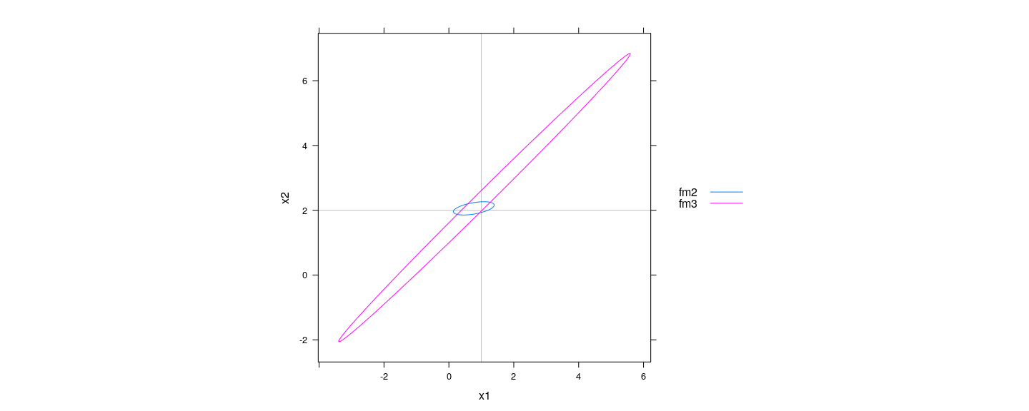
- Many different \((\beta_1, \beta_2, \beta_3)\) combinations give essentially equivalent fit
Variance inflation factor
- It can be shown that the sampling variance of \(\hat{\beta}_j\) is
\[ V( \hat{\beta}_j ) = \sigma^2 (\mathbf{X}^T \mathbf{X})^{-1}_{jj} = \frac{1}{1-R_j^2} \times \frac{\sigma^2}{(n-1) s_j^2} \]
where
\(s_j^2 = \frac{1}{n-1} \sum_i (X_{ij} - \bar{X}_j)^2\) (sample variance of \(X_{* j}\))
\(R_j^2\) is the multiple correlation coefficient of \(X_{* j}\) on the remaining columns of \(\mathbf{X}\)
Variance inflation factor
- The Variance Inflation Factor (VIF) is defined as
\[ VIF_j = \frac{1}{1-R_j^2} \]
\(VIF_j\) directly reflects the effect of collinearity on the precision of \(\hat{\beta}_j\)
Length of the confidence interval for \(\hat{\beta}_j\) is proportional to \(\sqrt{V(\hat{\beta}_j)}\), so more useful to compare \(\sqrt{VIF_j}\)
       x1        x2        x3
7.392177 12.581416 12.700439 x1 x2
1.040104 1.040104 Variance inflation factor
- For a more intuitive justification, recall partial regression of
- residuals from regression of \(\mathbf{y}\) on \(\mathbf{X}_{(-j)}\), and
- residuals from regression of \(\mathbf{X}_{*j}\) on \(\mathbf{X}_{(-j)}\)
\(\hat{\beta}_j\) from this partial regression is the same as \(\hat{\beta}_j\) from the full model
In presence of collinearity, residuals from regression of \(\mathbf{X}_{*j}\) on \(\mathbf{X}_{(-j)}\) will have very low variability
[1] 2.308524[1] 0.1817672Variance inflation factor
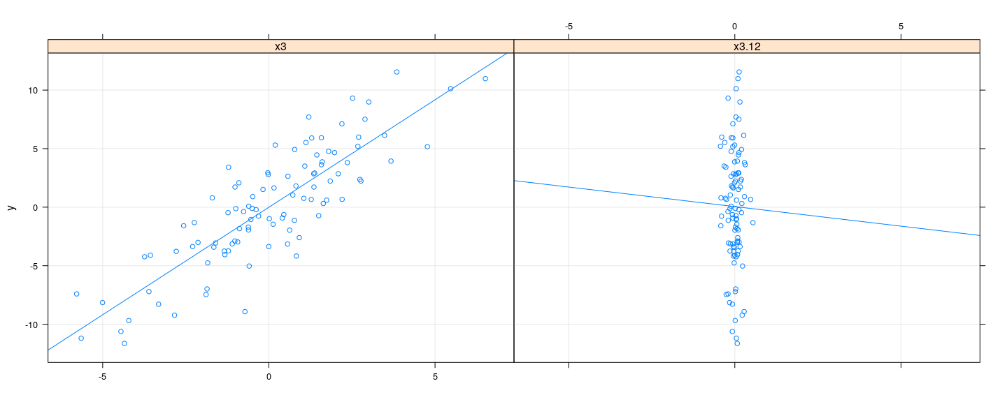
- Resulting \(\hat{\beta}_j\) is highly unstable
Coping with collinearity
There is no real solution if we want to estimate individual coefficients
Recall interpretation of \(\beta_j\): increase in \(E(y)\) for unit increase in \(x_j\) keeping other covariates fixed
For collinear data, this cannot be reliably estimated
However, there are several approaches to “stabilize” the model
Approaches to deal with collinearity
Variable selection:
- Use criteria such as AIC and BIC in conjunction with stepwise / all-subset search
- As discussed earlier, this is usually a misguided approach
- In presence of collinearity, choice of model very sensitive to random error
Respecify model: perhaps combine some predictors
- Principal component analysis (PCA):
- An automated version of model respecification
- Linearly transform covariates to make them orthogonal
- Reduce dimension of covariate space by dropping “unimportant” variables
Penalized regression:
- Add some sort of penalty for “unlikely” estimates of \(\beta\) (e.g., many large components)
- This is essentially a Bayesian approach
- Results in biased estimates, but usually much more stable
- For certain kinds of penalties, also works well as a variable selection mechanism
Standardization
We will briefly discuss principal components and penalized regression
Both these approaches have a practical drawback: they are not invariant to variable rescaling
Recall that for linear regression, location-scale changes of covariates does not change fitted model
This is no longer true if we used PCA or penalized regression
There is no real solution to this problem: usual practice is to standardize all covariates
Specifically, subtract mean, divide by standard deviation (so covariates have mean 0, variance 1)
For prediction, the same scaling must be applied to new observations
Can use R function
scale()which also returns mean and SD for subsequent useMore details later as necessary
Principal components
Will be studies in more details in Multivariate Analysis course
In what follows, the intercept is not considered as a covariate
Let \(\mathbf{z}_j\) denote the \(j\)-th covariate (column on \(\mathbf{X}\)) after standardization
This means that the length of each \(\mathbf{z}_j\) is \(\lVert \mathbf{z}_j \rVert = \sqrt{\sum_i z_{ij}^2} = n-1\)
This is not necessary for PCA, but is usually not meaningful
Consider the matrix \(\mathbf{Z} = [ \mathbf{z}_1 \, \mathbf{z}_2 \, \cdots \, \mathbf{z}_k ]\)
Suppose the rank of \(\mathbf{Z}\) is \(p\); for our purposes, \(p = k\)
Principal components
Our goal is to find \(\mathbf{W} = [ \mathbf{w}_1 \, \mathbf{w}_2 \, \cdots \, \mathbf{w}_p ] = \mathbf{Z} \mathbf{A}\) such that
\({\mathcal C}(\mathbf{W}) = {\mathcal C}(\mathbf{Z})\)
Columns of \(\mathbf{W}\) are mutually orthogonal
The first principal component \(\mathbf{w}_1\) has the largest variance among linear combinations of columns of \(\mathbf{Z}\)
The second principal component \(\mathbf{w}_2\) has the largest variance among linear combinations of columns of \(\mathbf{Z}\) that are orthogonal to \(\mathbf{w}_1\)
… and so on
More precisely, we only consider normalized linear combinations \(\mathbf{Z} \mathbf{a}\) such that \(\lVert \mathbf{a} \rVert^2 = \mathbf{a}^T \mathbf{a} = 1\)
Otherwise, the variance of \(\mathbf{Z} \mathbf{a}\) can be made arbitrarily large
Principal components
Note that by construction any linear combination of \(\mathbf{z}_1, \mathbf{z}_2, \dotsc, \mathbf{z}_k\) has mean 0
The variance of any such \(\mathbf{w} = \mathbf{Z} \mathbf{a}\) is given by
\[ s^2(\mathbf{a}) = \frac{1}{n-1} \mathbf{w}^T \mathbf{w} = \frac{1}{n-1} \mathbf{a}^T \mathbf{Z}^T \mathbf{Z} \mathbf{a} = \mathbf{a}^T \mathbf{R} \mathbf{a} \]
where \(\mathbf{R} = \frac{1}{n-1} \mathbf{Z}^T \mathbf{Z}\) is the correlation matrix of the original predictors \(\mathbf{X}\)
We can maximize \(s^2(\mathbf{a})\) subject to the constraint \(\mathbf{a}^T \mathbf{a} = 1\) using a Lagrange multiplier:
\[ F = \mathbf{a}^T \mathbf{R} \mathbf{a} - \lambda (\mathbf{a}^T \mathbf{a} - 1) \]
Principal components
- Differentiating w.r.t. \(\mathbf{a}\) and \(\lambda\) and equating to 0, we get
- In other words, potential solutions are the normalized eigenvectors of \(\mathbf{R}\)
Which of these \(k\) solutions maximizes \(s^2(\mathbf{a})\)?
For any solution \(\mathbf{a}\), the variance \(s^2(\mathbf{a}) = \mathbf{a}^T \mathbf{R} \mathbf{a} = \lambda\, \mathbf{a}^T \mathbf{a} = \lambda\)
So the first principal component is given by the eigenvector \(\mathbf{a}_1\) corresponding to the largest eigenvalue \(\lambda_1\)
Principal components
Let the eigenvalues in decreasing order be \(\lambda_1 \geq \lambda_2 \geq \cdots \geq \lambda_k\)
Not surprisingly, the principal components are given by the corresponding eigenvectors \(\mathbf{a}_1, \mathbf{a}_2, \dotsc, \mathbf{a}_k\)
The desired transformation matrix \(\mathbf{A}\) is given by \(\mathbf{A} = [ \mathbf{a}_1 \, \mathbf{a}_2 \, \cdots \, \mathbf{a}_k ]\)
As the eigenvectors are normalized, \(\mathbf{A}^T \mathbf{A} = \mathbf{I}\)
The variance-covariance matrix of the principal components \(\mathbf{W}\) is
\[ \frac{1}{n-1} \mathbf{W}^T \mathbf{W} = \frac{1}{n-1} \mathbf{A}^T \mathbf{Z}^T \mathbf{Z} \mathbf{A} = \mathbf{A}^T \mathbf{R} \mathbf{A} = \mathbf{A}^T \mathbf{A} \mathbf{\Lambda} = \mathbf{\Lambda} \]
- Here \(\mathbf{\Lambda}\) is the diagonal matrix with entries \(\lambda_1, \lambda_2, \dotsc, \lambda_k\)
Principal components
- A general indicator of the degree of collinearity present in the covariates is the condition number
\[ K \equiv \sqrt{\frac{\lambda_1}{\lambda_k}} \]
- Large condition number indicates that small changes in data can cause large changes in \(\hat{\beta}\)
In theory, using (all) principal components as covariates leads to the same fit (i.e., same \(\mathbf{H}\), \(\hat{\mathbf{y}}\), etc.)
To “stabilize” collinearity, we can instead regress on the first few principal components
Principal components in R
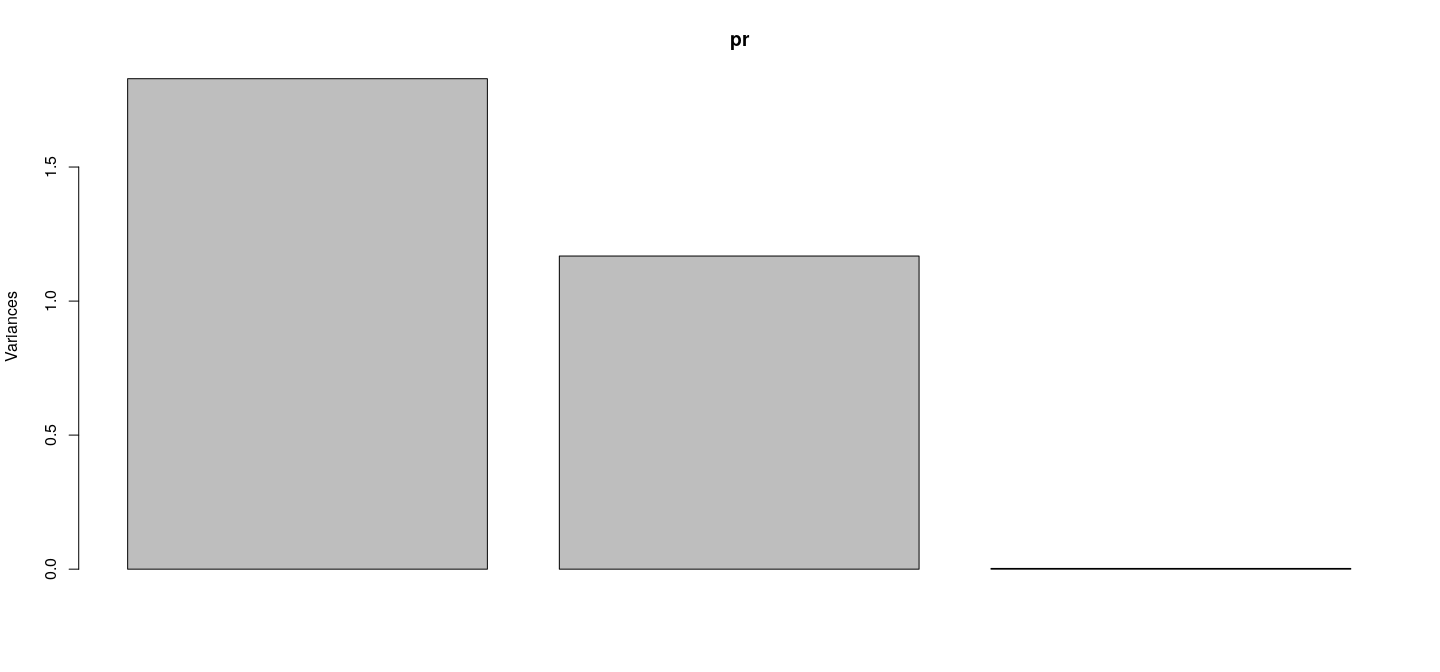
Standard deviations (1, .., p=3):
[1] 1.35254256 1.08071572 0.05178952

Rotation (n x k) = (3 x 3):
           PC1        PC2        PC3
x1 -0.02887707 -0.9244271  0.3802640
x2 -0.70174549  0.2896624  0.6508832
x3 -0.71184225 -0.2480529 -0.6570771 PC1 PC2 PC3
1 1.1023871 -0.0005434015 0.072144023
2 0.1583731 -1.9368798962 -0.023836194
3 -0.8266643 -0.1014248304 -0.088178195
4 0.3620938 0.6099882730 -0.020273616
5 1.2346433 0.2956850245 -0.023914456
6 1.7477325 1.2684577099 -0.002962102Principal components in R: scree plot
Principal components in R: biplot
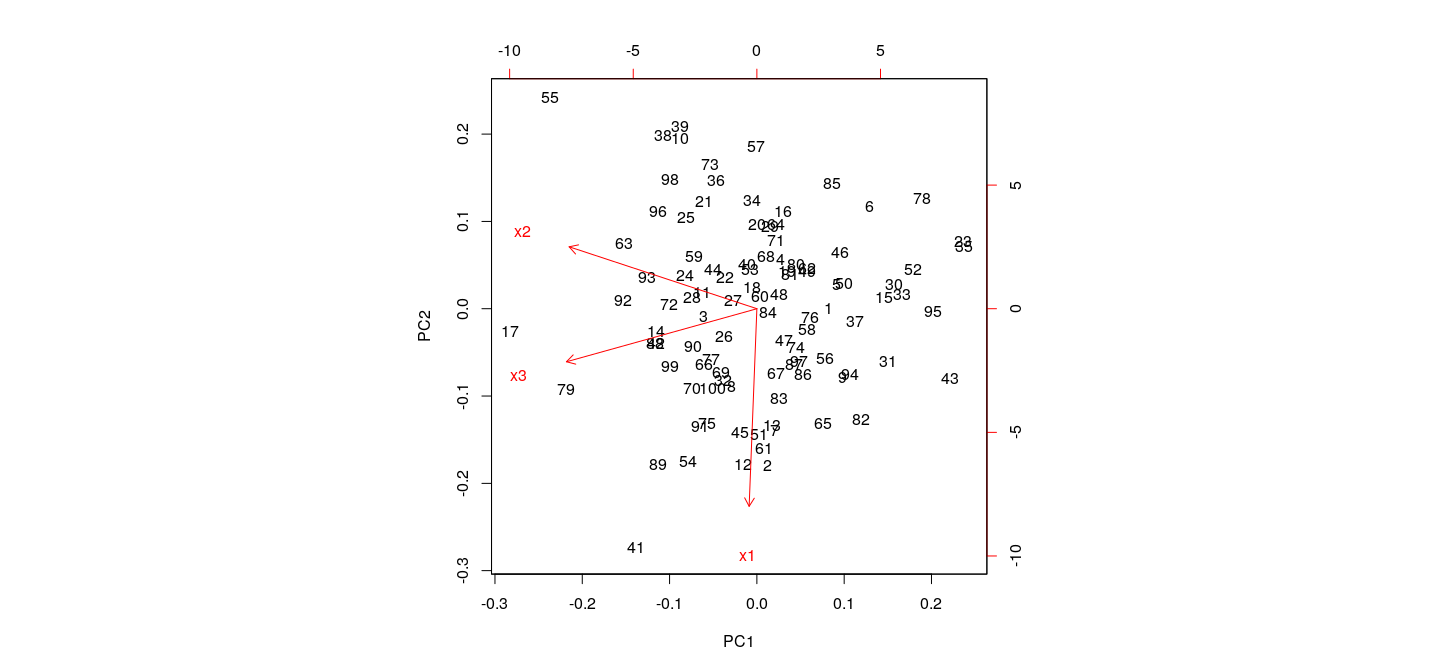
Principal components are orthogonal
Principal component regression
Call:
lm(formula = y ~ PC1 + PC2 + PC3, data = d3)

Residuals:
    Min      1Q  Median      3Q     Max
-4.5620 -1.3326 -0.0007  1.6717  4.5924

Coefficients:
            Estimate Std. Error t value Pr(>|t|)
(Intercept)  0.04883    0.20419   0.239    0.811
PC1         -3.35460    0.15173 -22.110   <2e-16 ***
PC2          0.41578    0.18989   2.190    0.031 *
PC3          4.65106    3.96249   1.174    0.243
---
Signif. codes:  0 '***' 0.001 '**' 0.01 '*' 0.05 '.' 0.1 ' ' 1

Residual standard error: 2.042 on 96 degrees of freedom
Multiple R-squared:  0.8376,    Adjusted R-squared:  0.8325
F-statistic: 165 on 3 and 96 DF, p-value: < 2.2e-16 (Intercept) PC1 PC2 PC3
(Intercept) 0.041692 0.000000 0.000000 0.00000
PC1 0.000000 0.023021 0.000000 0.00000
PC2 0.000000 0.000000 0.036058 0.00000
PC3 0.000000 0.000000 0.000000 15.70134Principal component regression
Call:
lm(formula = y ~ PC1 + PC2, data = d3)

Residuals:
    Min      1Q  Median      3Q     Max
-4.9339 -1.3878  0.0018  1.7533  4.3695

Coefficients:
            Estimate Std. Error t value Pr(>|t|)
(Intercept)  0.04883    0.20458   0.239   0.8118
PC1         -3.35460    0.15202 -22.067   <2e-16 ***
PC2          0.41578    0.19026   2.185   0.0313 *
---
Signif. codes:  0 '***' 0.001 '**' 0.01 '*' 0.05 '.' 0.1 ' ' 1

Residual standard error: 2.046 on 97 degrees of freedom
Multiple R-squared:  0.8352,    Adjusted R-squared:  0.8318
F-statistic: 245.9 on 2 and 97 DF, p-value: < 2.2e-16 (Intercept) PC1 PC2
(Intercept) 0.04185465 0.00000000 0.00000000
PC1 0.00000000 0.02311036 0.00000000
PC2 0.00000000 0.00000000 0.03619809Statistical interpretation of Principal Component regression
PCA rotates (through \(\mathbf{A}\)) and scales (through \(\mathbf{\Lambda}\)) \(\mathbf{Z}\) to make columns orthonormal
Resulting variables may be thought of as “latent variables” controlling observed covariates
Principal components with higher variability lead to smaller sampling variance of coefficients
Orthogonality means that estimated coefficients are uncorrelated
Unfortunately, no longer possible to interpret effect of individual covariates
- Confidence ellipsoids are essentially identical (except for different residual d.f.)
C3 <- chol(vcov(fm.pc3)[2:3, 2:3]) # only PC1 and PC2
C2 <- chol(vcov(fm.pc2)[2:3, 2:3])
tt <- seq(0, 1, length.out = 101)
circle <- rbind(2 * cos(2 * pi * tt), sin(2 * pi * tt))
E3 <- coef(fm.pc3)[2:3] + 2 * t(C3) %*% circle
E2 <- coef(fm.pc2)[2:3] + 2 * t(C2) %*% circle
E.pc <- as.data.frame(rbind(t(E2), t(E3))); E.pc$model <- rep(c("fm.pc2", "fm.pc3"), each = 101)
Confidence ellipsoids in principal component regression
xyplot(PC2 ~ PC1, data = E.pc, groups = model, abline = list(v = 1, h = 2, col = "grey"), type = "l",
       aspect = "iso", auto.key = list(lines = TRUE, points = FALSE, space = "right"))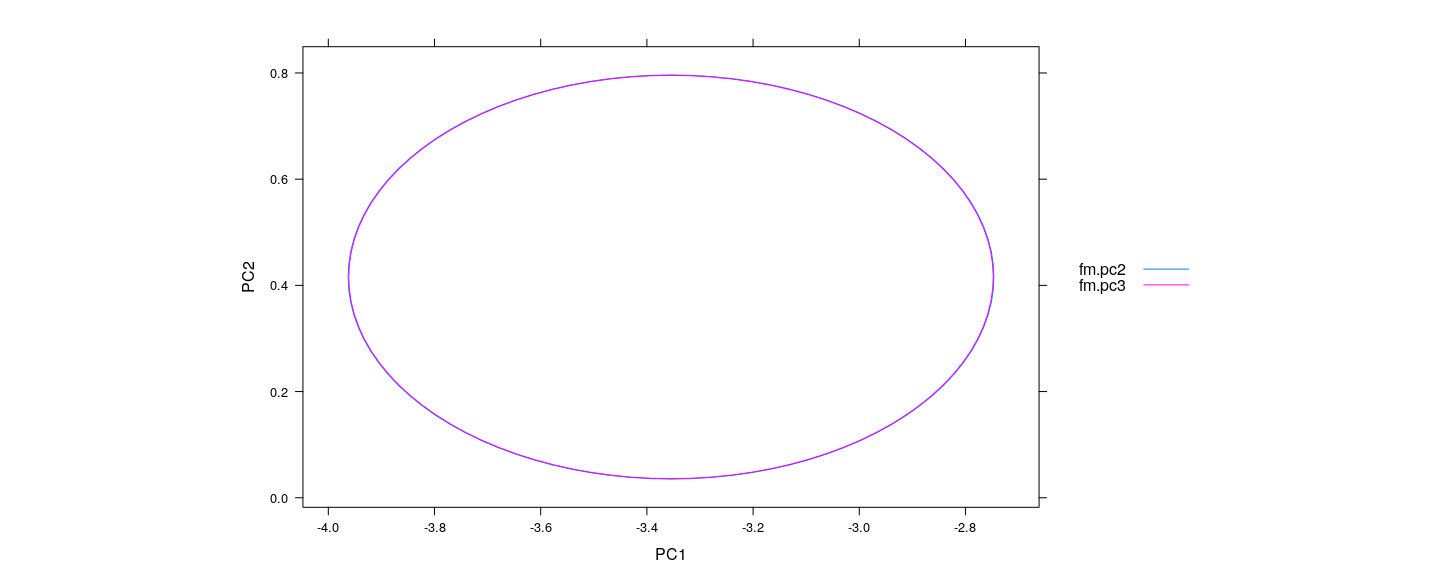
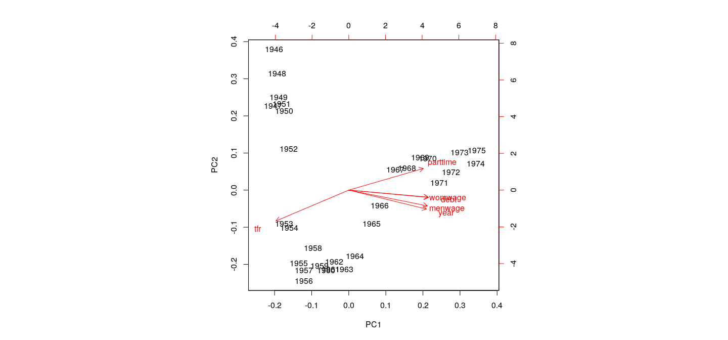
Example: Canadian Women’s Labour-Force Participation
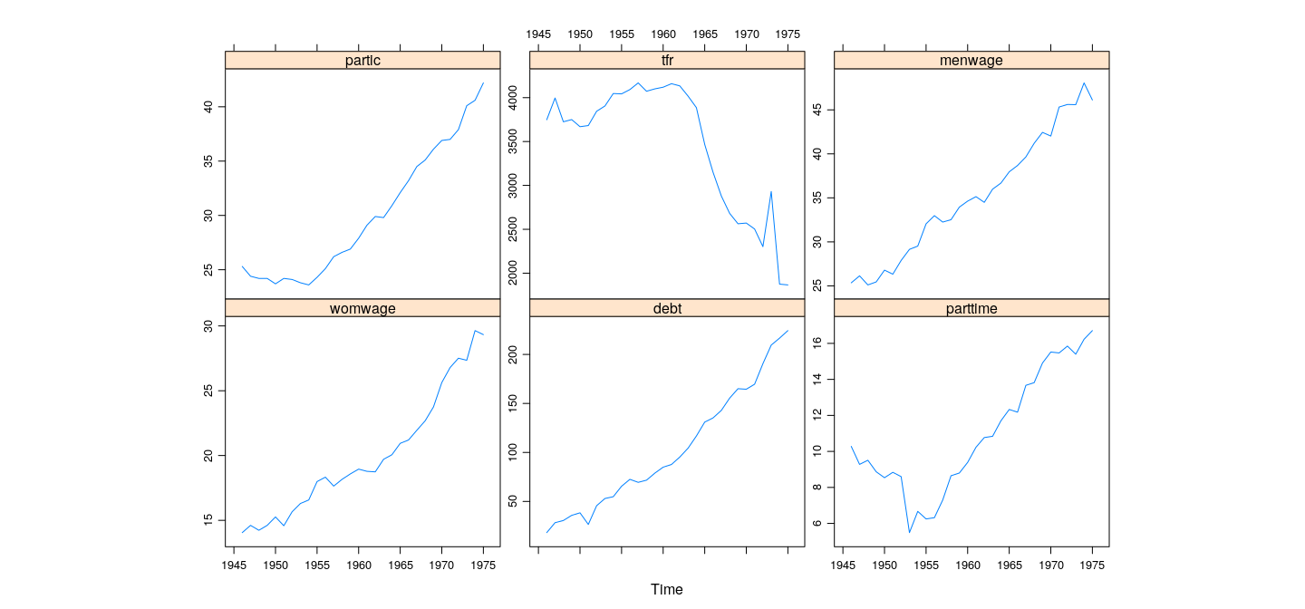
Example: Canadian Women’s Labour-Force Participation
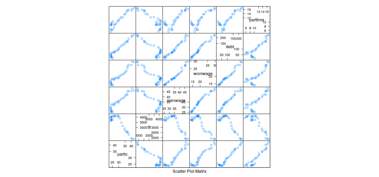
Example: Canadian Women’s Labour-Force Participation
Call:
lm(formula = partic ~ ., data = Bfox)

Residuals:
     Min       1Q   Median       3Q      Max
-0.83213 -0.33438 -0.01621  0.36769  1.05048

Coefficients:
              Estimate Std. Error t value Pr(>|t|)
(Intercept)  8.142e+00  2.129e+02   0.038  0.96982
tfr         -1.949e-06  5.011e-04  -0.004  0.99693
menwage     -2.919e-02  1.502e-01  -0.194  0.84766
womwage      1.984e-02  1.744e-01   0.114  0.91041
debt         6.397e-02  1.850e-02   3.459  0.00213 **
parttime     6.566e-01  8.205e-02   8.002 4.27e-08 ***
year         4.452e-03  1.107e-01   0.040  0.96827
---
Signif. codes:  0 '***' 0.001 '**' 0.01 '*' 0.05 '.' 0.1 ' ' 1

Residual standard error: 0.5381 on 23 degrees of freedom
Multiple R-squared:  0.9935,    Adjusted R-squared:  0.9918
F-statistic: 587.3 on 6 and 23 DF,  p-value: < 2.2e-16
Example: Canadian Women’s Labour-Force Participation
      tfr   menwage   womwage      debt  parttime      year
3.891829 10.673117 8.205214 11.474235 2.748158 9.755120 Standard deviations (1, .., p=6):
[1] 2.35180659 0.57341995 0.33183302 0.13614037 0.08403192 0.06698201
Rotation (n x k) = (6 x 6):
PC1 PC2 PC3 PC4 PC5 PC6
tfr -0.3849387 -0.6675739 0.54244962 0.2518053 0.19660094 0.09928673
menwage 0.4158879 -0.3420846 -0.02228191 0.1571042 -0.70548213 0.43258778
womwage 0.4195650 -0.1523080 -0.26579808 0.7291795 0.27909187 -0.34716538
debt 0.4220132 -0.1591200 -0.09747758 -0.2757411 0.61883636 0.57279338
parttime 0.3945669 0.4692796 0.77462008 0.1520461 0.02516761 0.01748999
year 0.4111526 -0.4105886 0.15831978 -0.5301495 -0.04646405 -0.59505293
Example: Canadian Women’s Labour-Force Participation
All variables contribute roughly equally to first PC
Note non-linear pattern (PCA only accounts for linear relationships)
Example: Canadian Women’s Labour-Force Participation
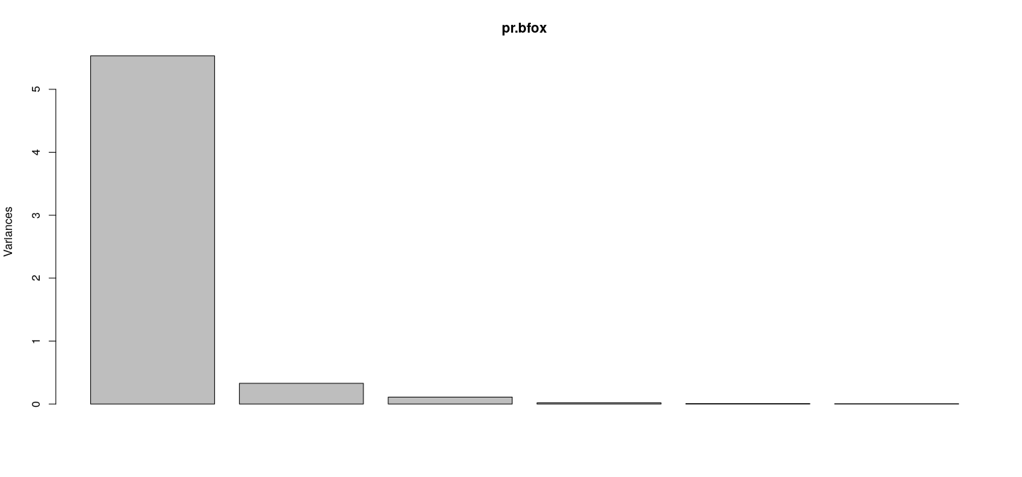
- First PC explains bulk of the variability (92%)
Example: Canadian Women’s Labour-Force Participation
Call:
lm(formula = partic ~ PC1 + PC2 + PC3 + PC4 + PC5 + PC6, data = Bfox)

Residuals:
     Min       1Q   Median       3Q      Max
-0.83213 -0.33438 -0.01621  0.36769  1.05048

Coefficients:
            Estimate Std. Error t value Pr(>|t|)
(Intercept) 29.99667    0.09823 305.356  < 2e-16 ***
PC1          2.50998    0.04248  59.080  < 2e-16 ***
PC2          0.44179    0.17424   2.535 0.018485 *
PC3          1.30075    0.30110   4.320 0.000254 ***
PC4         -0.74497    0.73391  -1.015 0.320632
PC5          2.67915    1.18900   2.253 0.034079 *
PC6          2.16416    1.49166   1.451 0.160326
---
Signif. codes:  0 '***' 0.001 '**' 0.01 '*' 0.05 '.' 0.1 ' ' 1

Residual standard error: 0.5381 on 23 degrees of freedom
Multiple R-squared:  0.9935,    Adjusted R-squared:  0.9918
F-statistic: 587.3 on 6 and 23 DF,  p-value: < 2.2e-16