Generalized Linear Models
Deepayan Sarkar
Motivation
- The standard linear model assumes
\[ y_i \sim N( \mathbf{x}_i^T \beta, \sigma^2) \]
In other words, the conditional distribution of \(Y | \mathbf{X} = \mathbf{x}\)
- is a normal distrbution
- with the mean parameter linear in terms involving \(x\), and
- the variance parameter independent of the mean
Generalized Linear Models (GLMs) allow the response distribution to be non-Normal
Still retains “linearity” in the sense that the conditional distribution depends on \(x\) only through \(\mathbf{x}_i^T \beta\)
Important special case: binary response
We will first focus on a special case: binary response
This problem can be viewed from various perspectives
Example:
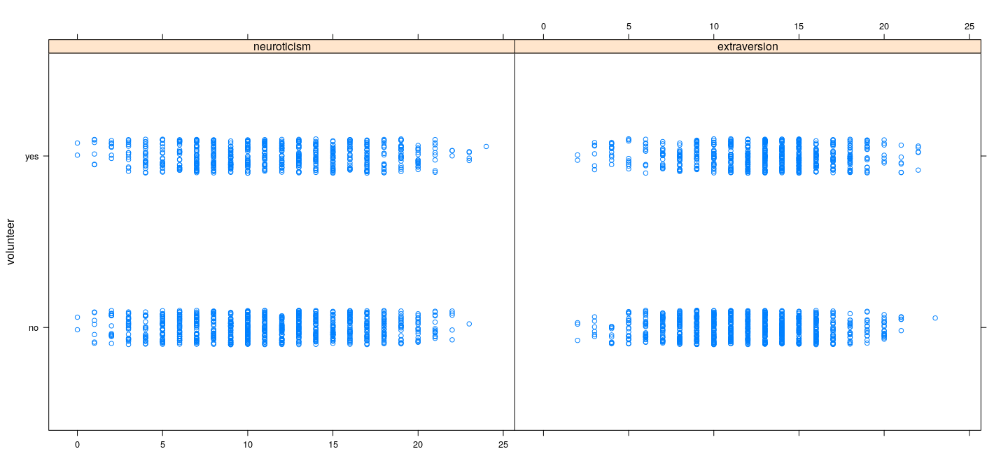
Cowlesdataset fromcarDatapackage (1421 rows):volunteer(response): whether willing to volunteer for psychological researchneuroticismas measured by a testextraversionas measured by a testsex: whether male or female
Interested in ‘predicting’ whether subject is willing to volunteer
Example: Data on volunteering
   neuroticism extraversion    sex volunteer
1           16           13 female        no
2            8           14   male        no
3            5           16   male        no
4            8           20 female        no
5            9           19   male        no
6            6           15   male        no
7            8           10 female        no
8           12           11   male        no
9           15           16   male        no
10          18            7   male        no
11          12           16 female        no
12           9           15   male        no
13          13           11   male        no
14           9           13   male        no
15          12           16 female        no
16          11           12   male        no
17           5            5   male        no
18          12            8   male        no
19           9            7   male        no
20           4           11 female        no
Example: Data on volunteering
Example: Data on volunteering
Example: Data on volunteering
Example: Data on volunteering
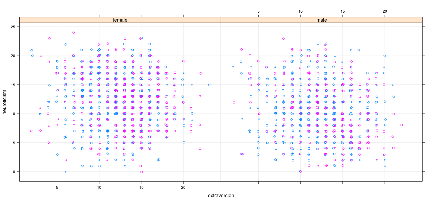
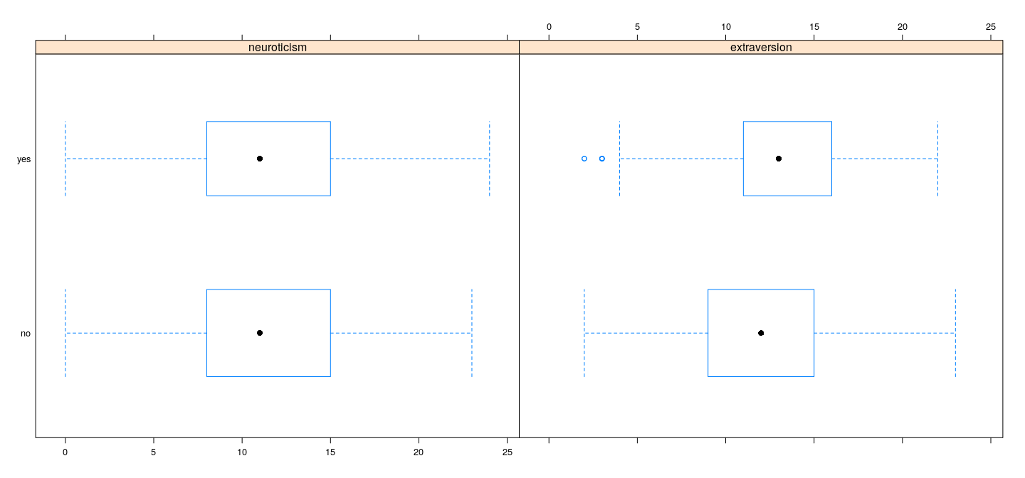
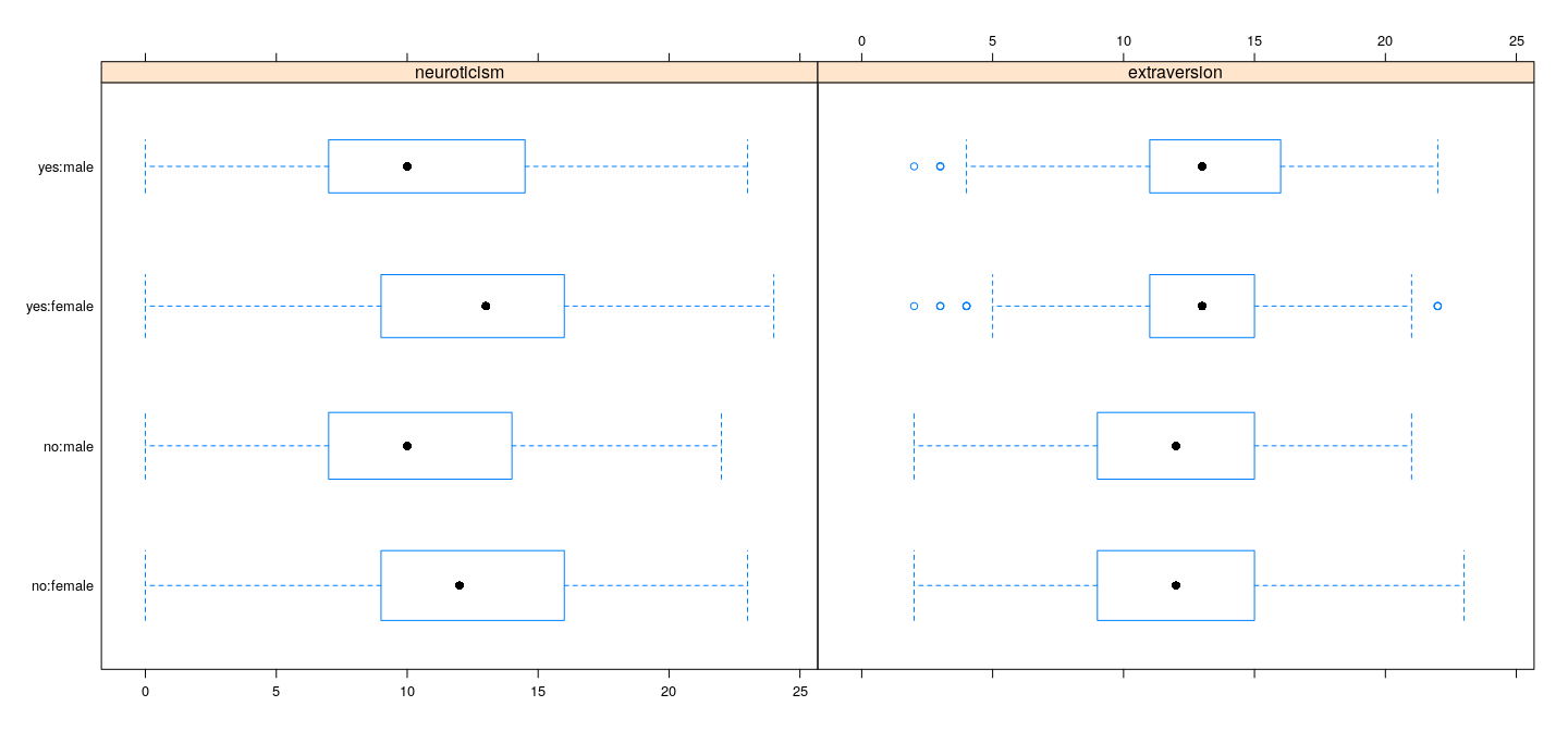
Summary
Dependence of response on predictors does not seem to be very strong
However, there is some information, and there appears to be some interaction
To proceed, we need to decide
- How can we predict willingness to volunteer?
- What is a suitable loss function?
Possible loss functions
- Loss based on conditional negative log-likelihood
- Needs a model for the conditional distribution of response
- Leads to GLM (logistic regression in this case)
Misclassfication loss (0 is correctly classified, 1 if misclassfied)
Even if we use GLM, this is often the loss function we are actually interested in
We will try some “simple” alternatives before we try logistic regression
Another example: Voting intentions in the 1988 Chilean plebiscite
Before proceeding, we look at another example where dependence is more clear-cut
Context: Chile was a military dictatorship under Augusto Pinochet from 1973–1990
- A referendum was held in October 1988 to decide if Chile should
- Continue with Pinochet (Yes; result: 45%)
- Return to democracy (No; result: 55%)
The
Chiledata (packagecarData): National survey conducted 5 months before the referendumResponse: intended vote (Yes / No / Abstain / Undecided)
Other variables are sex, age, income, etc., and
statusquowhich measures support for the status quo.
Example: Voting intentions data
xyplot(vote ~ age + jitter(log(income)) + statusquo, Chile, subset = vote %in% c("Y", "N"),
       outer = TRUE, jitter.y = TRUE, scales = list(x = "free"), xlab = NULL)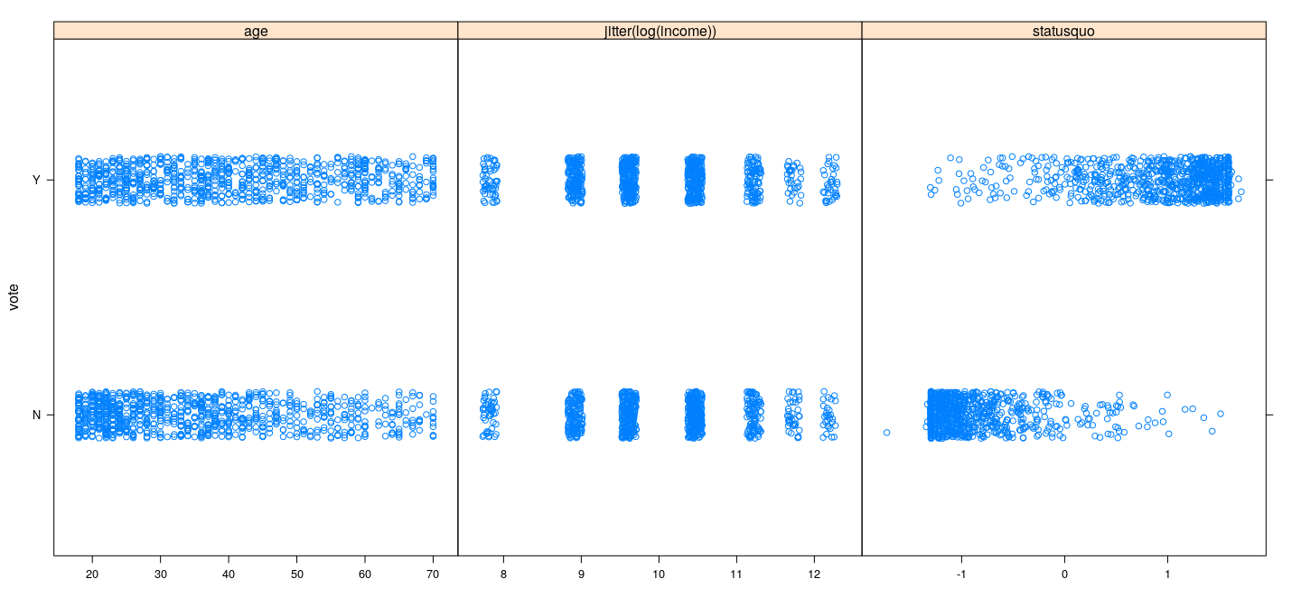
Mis-classification loss: goal is to minimize false classifications
Volunteering data
volunteer
 no yes
824 597 [1] 0.4201267Mis-classification loss: goal is to minimize false classifications
Voting intentions data
Chile <- droplevels(subset(Chile, vote %in% c("Y", "N"))) # remove Abstain / Undecided
(x <- xtabs(~ vote, Chile))
vote
N Y
889 868 [1] 0.4940239A simple non-parametric classification method: \(k\)-NN
Given \(x\), find \(k\) nearest neighbours
Classify as modal (most common) class among these \(k\) observations
Similar in spirit to LOWESS
library(class)
p <- knn.cv(Cowles[, "extraversion", drop = FALSE], cl = Cowles$volunteer, k = 11)
(x <- xtabs(~ p + Cowles$volunteer))
Cowles$volunteer
p no yes
no 673 429
yes 151 168[1] 0.4081633
- Slight improvement over baseline
A simple non-parametric classification method: \(k\)-NN
- More variables not necessarily better (worse than baseline)
p <- knn.cv(Cowles[, c("extraversion", "neuroticism")], cl = Cowles$volunteer, k = 11)
(x <- xtabs(~ p + Cowles$volunteer))
Cowles$volunteer
p no yes
no 628 436
yes 196 161[1] 0.4447572
A simple non-parametric classification method: \(k\)-NN
- Substantial improvement in voting intentions data
Chile2 <- subset(Chile, !(is.na(statusquo) | is.na(vote)))
p <- knn.cv(Chile2[, "statusquo", drop = FALSE], cl = Chile2$vote, k = 11)
(x <- xtabs(~ p + Chile2$vote))
Chile2$vote
p N Y
N 824 71
Y 64 795[1] 0.07696693
Many other classification approaches available (but not in the scope of this course)
We want to view this as a regression problem with a binary (0/1) response
A simple option: pretend that linear regression is valid
xyplot(volunteer ~ neuroticism + extraversion, Cowles, outer = TRUE, jitter.y = TRUE, xlab = NULL,
       type = c("p", "r", "smooth"), degree = 1, col.line = "black")
A simple option: pretend that linear regression is valid
xyplot(vote ~ age + jitter(log(income)) + statusquo, Chile,
       outer = TRUE, jitter.y = TRUE, scales = list(x = "free"), xlab = NULL,
       type = c("p", "r", "smooth"), degree = 1, col.line = "black")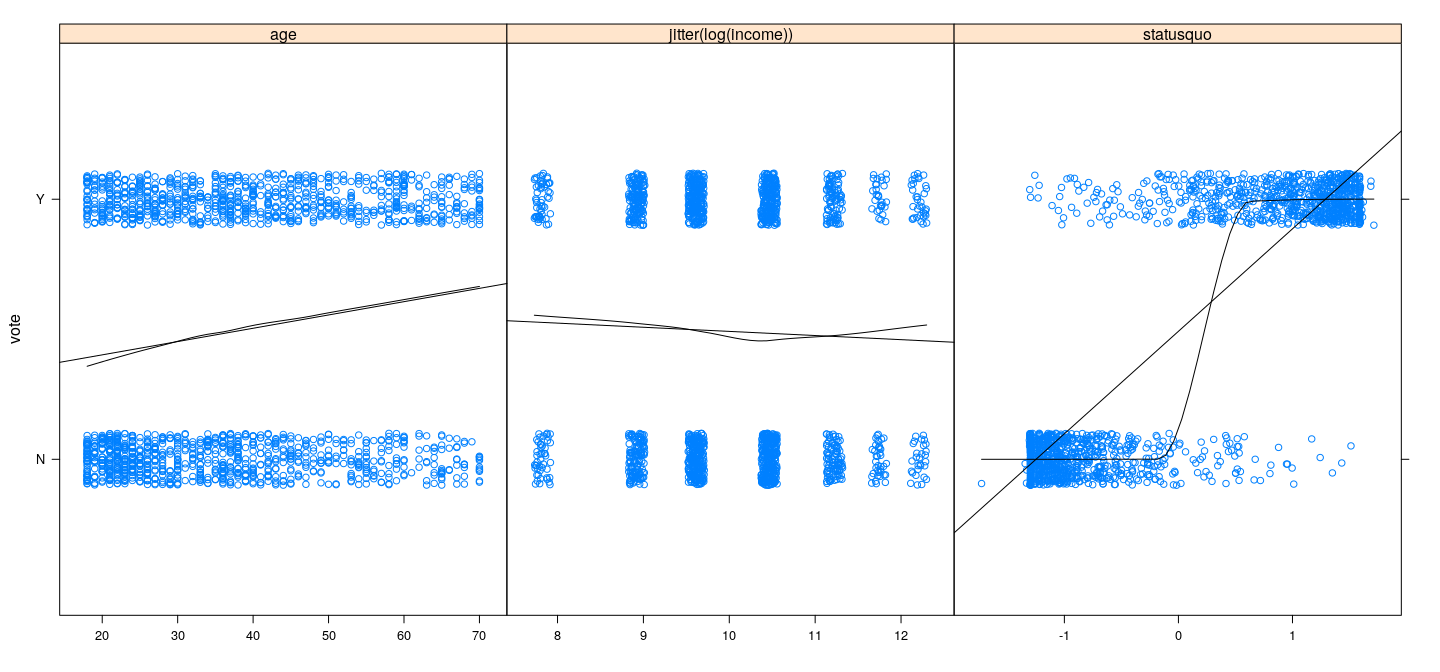
Can use linear regression to predict: volunteering
Cowles <- transform(Cowles, dvol = ifelse(volunteer == "no", 0, 1))
fm1 <- lm(dvol ~ extraversion, Cowles)
anova(fm1)
Analysis of Variance Table
Response: dvol
Df Sum Sq Mean Sq F value Pr(>F)
extraversion 1 5.32 5.3171 22.135 2.789e-06 ***
Residuals 1419 340.87 0.2402
---
Signif. codes: 0 '***' 0.001 '**' 0.01 '*' 0.05 '.' 0.1 ' ' 1 volunteer
predvol1 no yes
0 765 526
1 59 71[1] 0.4116819Can use linear regression to predict: volunteering
Analysis of Variance Table

Response: dvol
                   Df Sum Sq Mean Sq F value    Pr(>F)
neuroticism         1   0.06  0.0552  0.2298   0.63172
extraversion        1   5.49  5.4863 22.8623 1.922e-06 ***
sex                 1   1.07  1.0696  4.4571   0.03493 *
neuroticism:sex     1   0.02  0.0153  0.0640   0.80038
extraversion:sex    1   0.00  0.0006  0.0024   0.96109
Residuals        1415 339.56  0.2400
---
Signif. codes: 0 '***' 0.001 '**' 0.01 '*' 0.05 '.' 0.1 ' ' 1 volunteer
predvol2 no yes
0 745 512
1 79 85[1] 0.4159043Can use linear regression to predict: voting intentions
Chile <- transform(Chile, dvote = ifelse(vote == "N", 0, 1))
fm3 <- lm(dvote ~ statusquo, Chile, na.action = na.exclude)
anova(fm3)
Analysis of Variance Table
Response: dvote
Df Sum Sq Mean Sq F value Pr(>F)
statusquo 1 320.21 320.21 4745.2 < 2.2e-16 ***
Residuals 1752 118.23 0.07
---
Signif. codes: 0 '***' 0.001 '**' 0.01 '*' 0.05 '.' 0.1 ' ' 1 vote
predvote N Y
0 838 82
1 50 784[1] 0.07525656Can use linear regression to predict: voting intentions
Analysis of Variance Table

Response: dvote
            Df Sum Sq Mean Sq   F value Pr(>F)
statusquo    1 320.21  320.21 4747.5401 <2e-16 ***
age          1   0.13    0.13    1.8752 0.1711
Residuals 1751 118.10    0.07
---
Signif. codes: 0 '***' 0.001 '**' 0.01 '*' 0.05 '.' 0.1 ' ' 1 vote
predvote N Y
0 839 85
1 49 781[1] 0.07639681Drawbacks of linear regression
Model is clearly wrong: expected value should be in \([0, 1]\)
Expected value of response should be a non-linear function (of parameters)
Squared error is not a meaningful loss function
However, maximum likelihood approach is still reasonable
Natural response distribution is Bernoulli
Probability of “success” depends on covariates
Logistic regression assumes that this dependence is through a linear combination \(\mathbf{x}^T\beta\)
Model and terminology
- Model:
\[Y \vert X = x \sim Ber(\mu(x)) \text{ where } \mu: \mathbb{R}^p \to [0,1]\]
- Linear predictor
\[\eta = x^T \beta\]
- Link function \(g(\cdot)\):
\[\eta = g(\mu) \text{ where } g: [0,1] \to \mathbb{R}\]
- Inverse link function \(g^{-1}(\cdot)\) (also called the mean function):
\[\mu = g^{-1}(\eta) \text{ where } g^{-1}: \mathbb{R} \to [0,1]\]
Likelihood
Observations \((x_1, y_1), \dotsc, (x_n, y_n)\); linear predictors \(\eta_i = x_i^T \beta\); mean responses \(\mu_i = g^{-1}(\eta_i)\)
Likelihood
\[ \prod_{i=1}^n [g^{-1}(x_i^T \beta)]^{y_i} [1 - g^{-1}(x_i^T \beta)]^{1-y_i} = \prod_{i=1}^n \mu_i^{y_i} (1 - \mu_i)^{1-y_i} \]
- log-likelihood
\[ \sum_{i=1}^n [ y_i \log \mu_i + (1-y_i) \log (1 - \mu_i) ] \]
- log-likelihood for the simplest case of one predictor
\[ \sum_{i=1}^n [ y_i \log g^{-1}(\alpha + \beta x_i) + (1-y_i) \log (1 - g^{-1}(\alpha + \beta x_i)) ] \]
Will be completely specified once we specify the link function \(g(\cdot)\)
There are often multiple choices, with no reason to specifically prefer one over others
Choice of link function for binary response
The inverse link function \(g^{-1}(\eta)\) should have the following properties
- Should map \(\mathbb{R}\) to \([0, 1]\)
- Should be monotone (increasing, without loss of generality)
- Should decrease to 0 as \(\eta \to -\infty\), increase to 1 as \(\eta \to -\infty\)
These are properties satisfied by cumulative distribution functions
We are usually interested in smooth functions
Three particular choices are most commonly used:
- The logistic function \(\mu = \frac{e^\eta}{1 + e^\eta}\)
- The Normal CDF \(\mu = \Phi(\eta)\)
- The Cauchy CDF
The logistic function is also a CDF, although the corresponding distribution is not very common
It is a more “natural” choice in some sense, as we will see later
Common inverse link functions
logistic <- function(x) exp(x) / (1 + exp(x))
eta <- seq(-3, 3, 0.01)
xyplot(logistic(eta) + pnorm(eta) + pcauchy(eta) ~ eta, type = "l", ylab = NULL,
       auto.key = list(columns = 3, lines = TRUE, points = FALSE), grid = TRUE)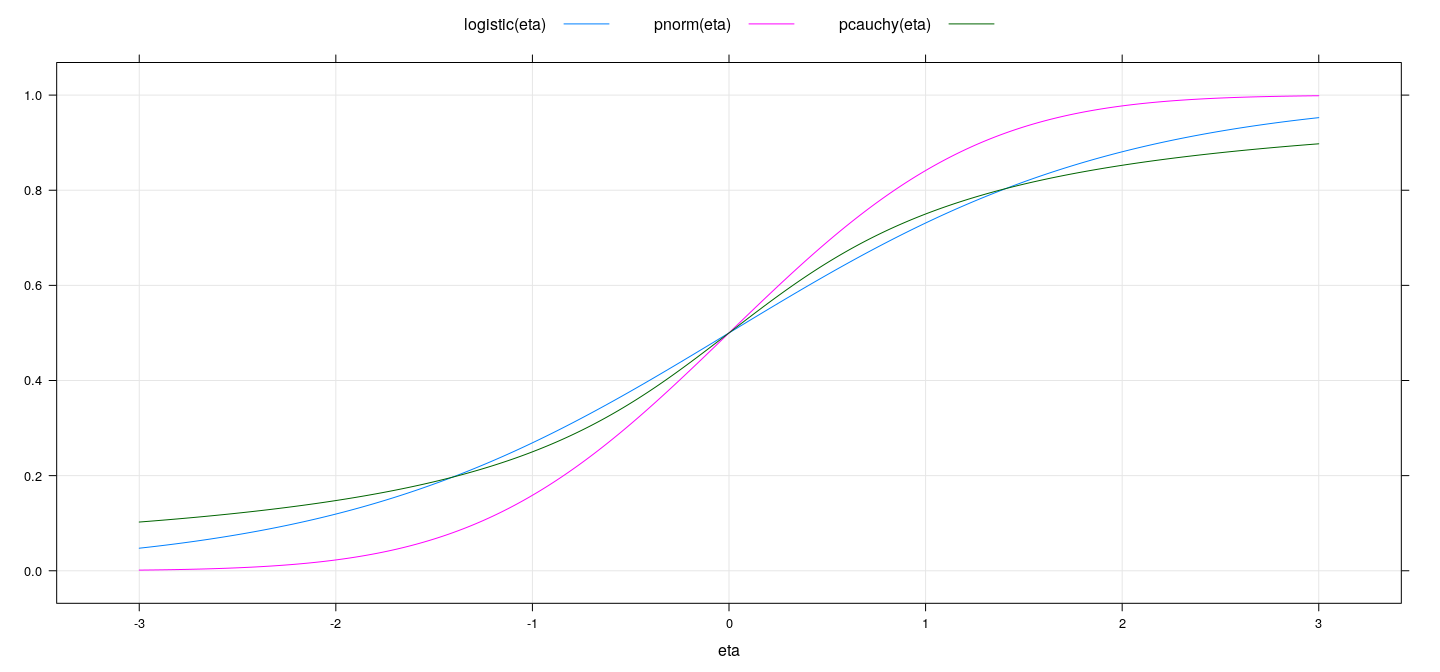
Common link functions
The corresponding link functions \(\eta = g(\mu)\) have standard names
Logit: \(\eta = \log \frac{\mu}{1-\mu}\)
Probit: \(\eta = \Phi^{-1} (\mu)\)
Cauchit: \(\eta = F^{-1} (\mu)\) where \(F\) is the Cauchy CDF
Link functions connect linear predictor \(\eta\) to mean response \(\mu\)
Choice of coefficients (e.g., \(\alpha\) and \(\beta\)) control location and slope
How can we estimate parameters?
We can think of this as a general optimization problem
Can be solved using general numerical optimizer (will see examples)
However, we study GLMs in detail for a different reason
For a specific but quite general class of distributions (exponential family)
- There is a simple and elegant way to estimate parameters
- Like M-estimation, this approach is an example of IRLS
- This allows tools developed for linear models to be easily adapted for GLMs
Examples revisited: volunteering data
- Before we study the general approach, let us try numerical optimization
negLogLik.logit <- function(beta)
{
    with(Cowles,
         {
             mu <- logistic(beta[1] + beta[2] * extraversion)
             -sum(dvol * log(mu) + (1-dvol) * log(1-mu))
         })
}
negLogLik.probit <- function(beta)
{
    with(Cowles,
         {
             mu <- pnorm(beta[1] + beta[2] * extraversion)
             -sum(dvol * log(mu) + (1-dvol) * log(1-mu))
         })
}
opt.logit <- optim(par = c(0, 1), fn = negLogLik.logit)
opt.probit <- optim(par = opt.logit$par, fn = negLogLik.probit)
opt.logit$par
[1] -1.14145947 0.06577276[1] -0.70500897 0.04048727Examples revisited: volunteering data
xyplot(dvol ~ extraversion, Cowles, jitter.x = TRUE, jitter.y = TRUE, ylim = c(-0.2, 1.2)) +
    layer(panel.curve(logistic(opt.logit$par[1] + opt.logit$par[2] * x), col = "black")) +
    layer(panel.curve(pnorm(opt.probit$par[1] + opt.probit$par[2] * x), col = "red"))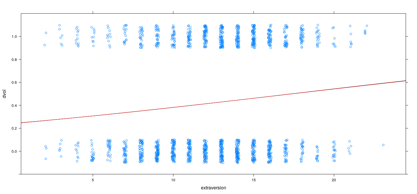
Examples revisited: volunteering data
pred.logit <- with(Cowles, logistic(opt.logit$par[1] + opt.logit$par[2] * extraversion) > 0.5)
(x <- xtabs(~ pred.logit + volunteer, Cowles))
volunteer
pred.logit no yes
FALSE 765 526
TRUE 59 71[1] 0.4116819pred.probit <- with(Cowles, logistic(opt.probit$par[1] + opt.probit$par[2] * extraversion) > 0.5)
(x <- xtabs(~ pred.probit + volunteer, Cowles)) volunteer
pred.probit no yes
FALSE 765 526
TRUE 59 71[1] 0.4116819Examples revisited: voting intentions data
negLogLik.logit <- function(beta)
{
    with(Chile,
         {
             mu <- logistic(beta[1] + beta[2] * statusquo)
             -sum(dvote * log(mu) + (1-dvote) * log(1-mu), na.rm = TRUE)
         })
}
negLogLik.probit <- function(beta)
{
    with(Chile,
         {
             mu <- pnorm(beta[1] + beta[2] * statusquo)
             -sum(dvote * log(mu) + (1-dvote) * log(1-mu), na.rm = TRUE)
         })
}
opt.logit <- optim(par = c(0, 1), fn = negLogLik.logit)
opt.probit <- optim(par = opt.logit$par, fn = negLogLik.probit)
opt.logit$par
[1] 0.2153074 3.2054346[1] 0.09379718 1.74529391Examples revisited: voting intentions data
xyplot(dvote ~ statusquo, Chile, jitter.y = TRUE, ylim = c(-0.2, 1.2)) +
    layer(panel.curve(logistic(opt.logit$par[1] + opt.logit$par[2] * x), col = "black")) +
    layer(panel.curve(pnorm(opt.probit$par[1] + opt.probit$par[2] * x), col = "red"))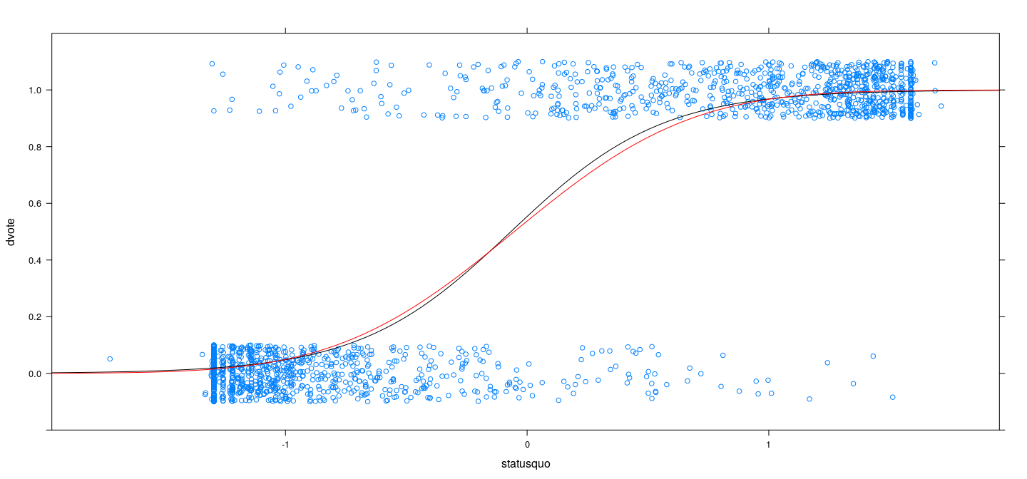
Examples revisited: voting intentions data
pred.logit <- with(Chile, logistic(opt.logit$par[1] + opt.logit$par[2] * statusquo) > 0.5)
(x <- xtabs(~ pred.logit + vote, Chile))
vote
pred.logit N Y
FALSE 829 76
TRUE 59 790[1] 0.07696693pred.probit <- with(Chile, logistic(opt.probit$par[1] + opt.probit$par[2] * statusquo) > 0.5)
(x <- xtabs(~ pred.probit + vote, Chile)) vote
pred.probit N Y
FALSE 829 76
TRUE 59 790[1] 0.07696693Inference: sampling distribution and testing
Inference approaches usually based on asymptotic properties of MLEs
In particular, estimates are asymptotically normal, and Wald tests are possible
Likelihood ratio tests can also be performed to compare models (asymptotically \(\chi^2\))
The general formulation: Exponential family
- A p.d.f. or p.m.f. of \(Y\) that can be written as
\[ p(y ; \theta, \varphi) = \exp \left[ \frac{y \theta - b(\theta)}{a(\varphi)} + c(y, \varphi) \right] \]
where
\(a(\cdot), b(\cdot), c(\cdot)\) are known functions; in most common cases, \(a(\varphi) = \varphi / a\) for some known \(a\)
\(\theta\) is known as the canonical parameter, and is essentially a location parameter
\(\varphi\) is a dispersion parameter (absent in some cases)
This representation can be made more general, but is sufficient (and more suitable) for our needs
The general formulation: Exponential family
Advantage: We can use general results for exponential families
Expectation and variance: it can be shown that
- \(E(Y) = \mu = b^\prime (\theta)\)
- \(V(Y) = \sigma^2 = b^{\prime\prime} (\theta) a(\varphi) = a(\varphi) v(\mu)\)
- In the simplified case, \(V(Y) = \varphi v(\mu) / a\)
In general, variance is function of mean (and possibly a dispersion parameter)
The function \(g_c(\cdot)\) such that \(\theta = g_c(\mu) = {b^\prime}^{-1}(\mu)\) is known as the canonical link function
Digression: expectation and variance of exponential family
- Using shorthand notation \(a \equiv a(\varphi)\) and \(c(y) = c(y, \varphi)\), we note that
\[ p(y) = \exp\left[ \frac{y \theta - b(\theta)}{a} + c(y) \right] = e^{-\frac{b(\theta)}{a}} \exp\left[ \frac{y \theta}{a} + c(y) \right] \]
- Assuming that \(p(y)\) is a density (analogous calculations are valid if \(p(y)\) is a mass function),
- Thus, we have
\[ \frac{b^{\prime}(\theta)}{a} = \frac{Q^{\prime}(\theta)}{Q(\theta)} \quad\text{ and }\quad \frac{b^{\prime\prime}(\theta)}{a} = \frac{Q^{\prime\prime}(\theta)}{Q(\theta)} - \left( \frac{Q^{\prime}(\theta)}{Q(\theta)} \right)^2 \]
Digression: expectation and variance of exponential family
- Now, interchanging \(\int\) and \(\frac{d}{d\theta}\) as necessary (Leibniz’s rule), we have
- It immediately follows that \(E(Y) = b^\prime(\theta)\) and \(V(Y) = a(\varphi) b^{\prime\prime}(\theta)\)
Examples of exponential families
| Family | \(a(\varphi)\) | \(b(\theta)\) | \(c(y, \varphi)\) |
|---|---|---|---|
| Gaussian | \(\varphi\) | \(\theta^2 / 2\) | \(-\frac12 [\frac{y^2}{\varphi} + \log (2\pi \varphi)]\) |
| Binomial proportion | \(1/n\) | \(\log (1 + e^{\theta})\) | \(\log {n \choose ny}\) |
| Poisson | \(1\) | \(e^\theta\) | \(-\log y!\) |
| Gamma | \(\varphi\) | \(-\log (-\theta)\) | \(\log (y/\varphi) / \varphi^2 - \log y - \log \Gamma(1/\varphi)\) |
| Inverse-Gaussian | \(\varphi\) | \(-\sqrt{-2 \theta}\) | \(-\frac12 [ \log (\pi \varphi y^3) + 1 / (\varphi y) ]\) |
Exercise: Verify
What are the corresponding canonical link functions?
GLM with response distribution given by exponential family
Observations \((x_i, y_i); i = 1, \dotsc, n\)
Basic premise of model: Location parameter \(\mu_i = E(Y | X = x_i)\) depends on predictors \(x_i\)
Variance depends on \(\mu_i\), but apart from that no dependence on predictors
In other words, dispersion parameter \(\varphi\) is a constant nuisance parameter
Dependence of \(\mu_i\) on \(x_i\) given by a link function \(g(\cdot)\) through the relationship
\[ g(\mu_i) = g(b^\prime(\theta_i)) = x_i^T \beta = \eta_i \]
- In other words, a GLM can be thought of as a linear model for the transformation \(g(\mu)\) of the mean \(\mu\)
If \(g(\cdot)\) is chosen to be the canonical link \(g_c(\cdot)\), then \(g(\mu_i) = \theta_i = x_i^T \beta = \eta_i\)
This choice leads to some simplications
However, no reason for effects of covariates to be additive on this particular (transformed) scale
Common link functions
| Link | \(\eta = g(\mu)\) | \(\mu = g^{-1}(\eta)\) |
|---|---|---|
| Identity | \(\mu\) | \(\eta\) |
| Log | \(\log \mu\) | \(e^\eta\) |
| Inverse | \(1/\mu\) | \(1/\eta\) |
| Inverse square | \(1/\mu^2\) | \(1/\sqrt{\eta}\) |
| Square root | \(\sqrt\mu\) | \(\eta^2\) |
| Logit | \(\log \frac{\mu}{1-\mu}\) | \(\frac{e^\eta}{1 + e^\eta}\) |
| Probit | \(\Phi^{-1}(\mu)\) | \(\Phi(\eta)\) |
| Log-log | \(-\log (-\log \mu)\) | \(e^{-e^{-\eta}}\) |
| Complementary log-log | \(\log (-\log \mu)\) | \(1 - e^{-e^\eta}\) |
- Last four are for Binomial proportion; last two are asymmetric (Exercise: plot and compare)
Comparison with variable transformation
GLM assumes that a transformation of the mean is linear in parameters
This is somewhat similar to transforming the response to achieve linearity in a linear model
However, in a linear model, transforming the response also changes its distribution / variance
In contrast, distribution of response and linearizing transformation are kept separate in GLM
- A practical problem: transformation may not be defined for all observations
- Bernoulli response \(0\) / \(1\) is mapped to \(\pm \infty\) by all link functions
- Poisson count of \(0\) is mapped to \(-\infty\) by \(\log\) link
Maximum likelihood estimation
- Log-likelihood (assuming for the moment that \(a(\varphi)\) may depend on \(i\))
\[ \ell(\theta(\beta), \varphi | y) = \log L(\theta(\beta), \varphi | y) = \sum_{i=1}^n \left[ \frac{y_i \theta_i - b(\theta_i)}{a_i(\varphi)} + c(y_i, \varphi) \right] = \sum_{i=1}^n \ell_i \]
Suppose link function is \(g(\mu_i) = \eta_i = x_i^T \beta\) where \(\mu_i = b^\prime(\theta_i)\)
To obtain score equations / estimating equations, we need to calculate (for \(i = 1, \dotsc, n; j = 1, \dotsc, p\))
\[ \frac{\partial \ell_i}{\partial \beta_j} = \frac{\partial \ell_i}{\partial \theta_i} \times \frac{\partial \theta_i}{\partial \mu_i} \times \frac{\partial \mu_i}{\partial \eta_i} \times \frac{\partial \eta_i}{\partial \beta_j} \]
- Note that \(b^{\prime}(\theta_i) = \mu_i\), \(\frac{\partial \mu_i}{\partial \theta_i} = b^{\prime\prime}(\theta_i) = v(\mu_i)\), \(\frac{\partial \eta_i}{\partial \mu_i} = g^{\prime}(\mu_i)\), and \(\frac{\partial \eta_i}{\partial \beta_j} = x_{ij}\)
Maximum likelihood estimation
- After simplification, we obtain the score equations (one for each \(\beta_j\))
\[ s_j(\beta) = \frac{\partial}{\partial \beta_j} \ell(\theta(\beta), \varphi | y) = \sum_{i=1}^n \frac{y_i - \mu_i}{a_i(\varphi) v(\mu_i)} \times \frac{x_{ij}}{g^{\prime}(\mu_i)} = 0 \]
- To proceed further, we need to assume the form \(a_i(\varphi) = \varphi / a_i\), which gives
\[ s_j(\beta) = \sum_{i=1}^n \frac{a_i (y_i - \mu_i)}{v(\mu_i)} \times \frac{x_{ij}}{g^{\prime}(\mu_i)} = 0 \]
In other words, score equations for \(\beta\) do not depend on the dispersion parameter \(\varphi\)
In practice, \(a_i\) is constant for most models; for binomial proportion, \(\varphi = 1\) and \(a_i = n_i\)
Maximum likelihood estimation with canonical link
- Further simplification when \(g(\cdot)\) is the canonical link \(g_c(\cdot)\), where \(\eta_i = \theta_i\)
\[ \frac{\partial \ell_i}{\partial \beta_j} = \frac{\partial \ell_i}{\partial \theta_i} \times \frac{\partial \eta_i}{\partial \beta_j} = \frac{y_i - \mu_i}{a_i(\theta)} x_{ij} \]
- Score equations become (when \(a_i(\varphi) = \varphi/a_i\))
\[ \sum_{i=1}^n a_i y_i x_{ij} = \sum_{i=1}^n a_i \mu_i x_{ij} \]
Analogy with normal equations in linear model
- With \(\mathbf{A} = diag(a_1, \dotsc, a_n)\) diagonal matrix of prior weights, these can be written as
\[ \mathbf{X}^T \mathbf{A} \mu(\beta) = \mathbf{X}^T \mathbf{A} \mathbf{y} \]
- In particular, when \(\mathbf{A} = \mathbf{I}\) (for Binomial, use individual Bernoulli trials)
\[ \mathbf{X}^T (\mathbf{y} - \hat\mu) = \mathbf{0} \]
In other words, “residuals” are orthogonal to column space of \(\mathbf{X}\)
In the linear model, \(\mu(\beta) = \mathbf{X} \beta\), giving the usual normal equations
In general, the score equations are non-linear in \(\beta\) because \(\mu(\beta)\) is non-linear
This is true whether or not we use the canonical link
How can we solve them? Need some kind of iterative method
Digression: Newton-Raphson and Fisher scoring
The Newton-Raphson method is a general numerical algorithm to solve \(f(x) = 0\)
Suppose we have an approximate solution \(x_0\)
Locally approximate \(f(x)\) by a line (first order Taylor series approximation)
\[ f(x) \approx f(x_0) + f^\prime(x_0) (x-x_0) \]
- A hopefully “closer” solution of \(f(x) = 0\) is the root of this approximation
\[ x_1 = x_0 - \frac{f(x_0)}{f^\prime(x_0)} \]
- Treat \(x_1\) as an updated estimate and iterate until convergence
\[ x^{(t+1)} = x^{(t)} - \frac{f(x^{(t)})}{f^\prime(x^{(t)})} \]
- This usually works as long as we get a good starting estimate \(x^{(0)}\) and \(f\) is well behaved
Digression: Newton-Raphson and Fisher scoring
In our case, \(f\) is the score function \(s(\beta)\)
This is actually a set of \(p\) separate equations \(s_j(\beta) = 0\) (one for each \(\beta_j\))
In other words, \(s(\cdot)\) is a vector function
\[ s: \mathbb{R}^p \to \mathbb{R}^p \]
- Fortunately, the algorithm is still valid, giving
\[ \hat{\beta}^{(t+1)} = \hat{\beta}^{(t)} - \left( H\left(\hat{\beta}^{(t)}\right) \right)^{-1} s(\hat{\beta}^{(t)}) \]
where \(H\left(\hat{\beta}^{(t)}\right)\) is the Jacobian matrix of \(s(\cdot)\) or the Hessian of the log-likelihood function at \(\hat{\beta}^{(t)}\)
The only potential difficulty is in computing \(H\)
Digression: Newton-Raphson and Fisher scoring
In the context of maximum likelihood estimation, \(H\) is closely related to Fisher information
Recall that for a scalar parameter \(\theta\),
\[ E_\theta(s(\theta; X)) = E_\theta \left[ \frac{\partial}{\partial \theta} \log f(X; \theta) \right] = \int \frac{\frac{\partial}{\partial \theta} f(x; \theta)}{f(x; \theta)} f(x; \theta) = \frac{\partial}{\partial \theta} 1 = 0 \]
- Also, under regularity conditions, the variance of the score function (a.k.a. Fisher information) is given by
\[ I(\theta) = V_\theta(s(\theta; X)) = E_\theta \left[ \left( \frac{\partial}{\partial \theta} \log f(X; \theta) \right)^2 \right] = -E_{\theta} \left[ \frac{\partial^2}{\partial \theta^2} \log f(X; \theta) \right] = -E_{\theta} H(\theta; X) \]
In other words, Fisher information is the expected value of the Hessian
\(-H(\theta; X)\) is often referred to as the observed information (as it depends on the observations \(X\))
Digression: Newton-Raphson and Fisher scoring
These results hold for vector-valued parameters as well
The Newton-Raphson algorithm described above uses the observed information
If we use Fisher information instead, we get the so-called “Fisher scoring” algorithm
Before we try to see how this turns out, we look at a more “intuitive” iterative method
Iteratively Reweighted Least Squares for GLM
Write \(y = \mu + (y-\mu) = \mu + \epsilon\). Can we transform both \(\mu\) and \(\epsilon\) to the linear scale?
\(\eta = g(\mu)\) is the “mean” in the linear scale, and a first order Taylor approximation of \(g\) around \(\mu\) gives
\[ \tilde{g}(y) = g(\mu) + g^{\prime}(\mu) (y - \mu) \]
- Use this to define “error” \(\varepsilon_i\) and “response” \(z_i\) on the linear scale as
\[ z_i \equiv \tilde{g}(y_i) = g(\mu_i) + g^{\prime}(\mu_i) (y_i - \mu_i) = \eta_i + \varepsilon_i \]
- It follows that
\[ E(z_i) = \eta_i = x_i^T \beta \quad\text{ and }\quad V(z_i) = [ g^\prime(\mu_i) ]^2 v(\mu_i) / a_i \]
This is a weighted linear model that can be fitted using weighted least squares problem…
apart from the slight inconvenience that \(\mu_i\)-s depend on the unknown parameter \(\beta\)
Iteratively Reweighted Least Squares for GLM
However, this immediately suggests the following iterative approach:
Start with initial estimates \(\hat{\mu}^{(0)}_i\) and \(\hat{\eta}^{(0)}_i = g(\hat{\mu}^{(0)}_i)\)
- For each iteration, set
- working response \(z^{(t)}_i = \hat{\eta}^{(t)}_i + g^{\prime}(\hat{\mu}^{(t)}_i) \left( y_i - \hat{\mu}^{(t)}_i \right)\)
- working weights \[w^{(t)}_i = \frac{a_i}{\left[ g^\prime(\hat{\mu}^{(t)}_i) \right]^2 v(\hat{\mu}^{(t)}_i)}\]
Fit a weighted least squares model for \(\mathbf{z}\) on \(X\) with weights \(\mathbf{w}\) to obtain \(\hat{\beta}^{(t+1)}\)
Define \(\hat{\eta}^{(t+1)}_i = x_i^T \hat{\beta}^{(t+1)}\) and \(\hat{\mu}^{(t+1)}_i = g^{-1}\left( \hat{\eta}^{(t+1)}_i \right)\)
Repeat steps 2–4 until convergence
Iteratively Reweighted Least Squares for GLM
- In matrix notation, the iteration can be written as
- Where
- \(W^{(t)}\) is a diagonal matrix with elements \(w_i^{(t)}\)
- \(\tilde{G}^{(t)}\) is a diagonal matrix with elements \(g^{\prime}( \hat\mu_i^{(t)} )\)
It turns out that this is equivalent to the Fisher scoring algorithm
Enough to show
\[ (X^T W^{(t)} X)^{-1} X^T W^{(t)} \tilde{G}^{(t)} \, (\mathbf{y} - \hat\mu^{(t)}) = - \left( E_{\beta} H\left(\hat{\beta}^{(t)}\right) \right)^{-1} s(\hat{\beta}^{(t)}) \]
- Additionally, with the canonical link, this reduces to the Newton-Raphson algorithm
Calculation of Hessian \(H\)
- Recall that
\[ \frac{\partial \ell_i}{\partial \theta_i} = \frac{y_i - b^\prime(\theta_i)}{a_i(\varphi)} \implies \frac{\partial^2 \ell_i}{\partial \theta_i^2} = \frac{\partial }{\partial \theta_i} \left( \frac{y_i - \mu_i}{a_i(\varphi)} \right) = \frac{-b^{\prime\prime}(\theta_i)}{a_i(\varphi)} = -\frac{v(\mu_i)}{a_i(\varphi)} \]
- \(H_{jk} = \sum_i h_{ijk}\), where
Calculation of Hessian \(H\) when \(g(\cdot)\) is canonical link
\(\frac{\partial \theta_i}{\partial \mu_i} \times \frac{\partial \mu_i}{\partial \eta_i} \equiv 1\)
First term vanishes
Second term does not involve observations \(y_i\)
Observed information equals expected information
Results in Newton-Raphson iterations
Hessian is given by
\[ H_{jk} = - \sum_{i=1}^n \frac{v(\mu_i)}{a_i(\varphi)} x_{ij} x_{ik} \]
Calculation of expected Hessian \(H\) for general link
First term vanishes after taking expectation as \(E_{\beta}(y_i - \mu_i) = 0\) (second term does not involve \(y\))
Results in Fisher scoring iterations (Newton-Raphson possible, but not equivalent to IRLS)
Second term simplifies as before
Expected Hessian is given by (after assuming \(a_i(\varphi) = \varphi / a_i\))
\[ E_{\beta}H_{jk} = - \sum_{i=1}^n \frac{v(\mu_i)}{a_i(\varphi)} \left( \frac{1}{v(\mu_i) g^\prime(\mu_i)} \right)^2 x_{ij} x_{ik} = - \sum_{i=1}^n \frac{a_i}{ [g^\prime(\mu_i)]^2 v(\mu_i) } x_{ij} x_{ik} \]
- In other words, Fisher information \(I = -E_{\beta} H = X^T W X\), where \(W\) is diagonal with entries
\[ w_i = \frac{a_i}{ [g^\prime(\mu_i)]^2 v(\mu_i)} \]
Equivalence of Fisher scoring and IRLS
- Recall: We need to show that
\[ (X^T W^{(t)} X)^{-1} X^T W^{(t)} \tilde{G}^{(t)} \, (\mathbf{y} - \hat\mu^{(t)}) = - \left( E_{\beta} H\left(\hat{\beta}^{(t)}\right) \right)^{-1} s(\hat{\beta}^{(t)}) \]
We have just shown that \(X^T W^{(t)} X = -E_{\beta} H\left(\hat{\beta}^{(t)}\right)\)
Remains to show that \(X^T W^{(t)} \tilde{G}^{(t)} \, (\mathbf{y} - \hat\mu^{(t)}) = s(\hat{\beta}^{(t)})\)
Dropping the suffix \(^{(t)}\) indicating iteration, the \(j\)-th element of the RHS is
\[ s(\beta) = \sum_{i=1}^n \frac{a_i (y_i - \mu_i)}{v(\mu_i)} \cdot \frac{x_{ij}}{g^{\prime}(\mu_i)} = \sum_{i=1}^n x_{ij} \left[ \frac{a_i }{ [g^{\prime}(\mu_i)]^2 v(\mu_i)} \cdot g^{\prime}(\mu_i) \right] (y_i - \mu_i) \]
- It is easy to see that the \(j\)-th element of the LHS is the same
Initial estimates
Simple choice: \(\hat{\mu}^{(0)}_i = y_i\)
- This may cause a problem computing \(\hat{\eta}^{(0)}_i\) in some cases
- For Bernoulli response, if \(\mu = y \in \{0,1\}\), logit\((\mu) = \pm \infty\)
- For Poisson response, if \(\mu = y = 0, \log(\mu) = -\infty\)
The initial values are not that critical, and can be adjusted to avoid this
E.g., choose initial \(\mu = 0.5\) for Bernoulli, or \(\mu = 1\) when \(y = 0\) for Poisson
Estimating the dispersion parameter
Recall that \(V(y_i) = \varphi v(\mu_i) / a_i\)
This suggests the method of moments estimator
\[ \hat{\varphi} = \frac{1}{n-p} \sum_{i=1}^n \frac{ a_i (y_i - \hat{\mu}_i)^2 }{v(\hat{\mu}_i)} \]
- This is usually preferred over the MLE of \(\varphi\)
Asymptotic sampling distribution of \(\hat\beta\)
Under mild regularity conditions, the MLE \(\hat\beta\) is asymptotically normal
Variance-covariance matrix is given by inverse of Fisher information
\[\hat\beta \sim AN(\beta, \varphi \, I_{\mu}^{-1} ) \equiv AN(\beta, \varphi \, \left( X^T W_\mu X \right)^{-1}) \]
- So Wald tests for linear functions of \(\beta\) can be performed using standard errors based on
\[\hat{V}(\hat\beta) = \hat\varphi \, \left( X^T W_{\hat\mu} X \right)^{-1}\]
For models without a dispersion parameter, these are approximate \(\chi^2\) or \(z\)-tests
For models with a dispersion parameter, these are approximate \(F\) or \(t\)-tests
Analysis of deviance
\(F\)-tests to test nested models in linear regression are no longer valid
Analogous tests can be performed using asymptotic results for likelihood ratio tests
Recall that the log-likelihood for the model can be written as
\[ \ell(\mu, \varphi | y) = \log L(\mu, \varphi | y) = \sum_{i=1}^n \left[ \frac{a_i (y_i \theta_i - b(\theta_i))}{\varphi} + c(y_i, \varphi) \right] \]
- For any fitted model, this can be compared with the “saturated model” \(\hat\mu_i = y_i\)
Analysis of deviance
- Define deviance (ignoring the dispersion parameter) as twice the difference in log-likelihoods
Boundary problems can be resolved on the observation scale
This is analogous to sum of squared errors in a linear model (exercise: check for Gaussian)
Forms basis for (asymptotic) \(\chi^2\) tests for models without a dispersion parameter (Binomial, Poisson)
Exercise: Compute deviance explicitly for Binomial proportion and Poisson
Analysis of deviance
- The scaled deviance divides by the estimated dispersion parameter
\[ D^{*}(y; \hat\mu) = D(y; \hat\mu) / \hat\varphi \]
Forms basis for (approximate) \(F\) tests for models with a dispersion parameter
The deviance for a constant mean model (intercept only) is called the null deviance (say \(D_0\))
A GLM analogue of the coefficient of determination \(R^2\) for a model with deviance \(D_1\) is
\[ R^2 = 1 - \frac{D_1}{D_0} \]
Fitting Generalized Linear Models in R
GLMs are fit using the function
glm(), which has an interface similar tolm()In addition to a formula and the
dataargument,glm()requires afamilyargument to be specifiedExamples (continuous):
Fitting Generalized Linear Models in R
GLMs are fit using the function
glm(), which has an interface similar tolm()In addition to a formula and the
dataargument,glm()requires afamilyargument to be specifiedExamples (discrete):
Fitting Generalized Linear Models in R
- The link function can also be constructed by specifying the functions
link: \(g\)linkinv: \(g^{-1}\)mu.eta: \(\frac{d\mu}{d\eta}\)
List of 5
 $ linkfun :function (mu)
 $ linkinv :function (eta)
 $ mu.eta  :function (eta)
 $ valideta:function (eta)
 $ name    : chr "probit"
 - attr(*, "class")= chr "link-glm"
Example: volunteering
fgm1 <- glm(dvol ~ (extraversion + neuroticism) * sex, Cowles, family = binomial("logit"))
summary(fgm1)
Call:
glm(formula = dvol ~ (extraversion + neuroticism) * sex, family = binomial("logit"),
    data = Cowles)

Deviance Residuals:
    Min       1Q   Median       3Q      Max
-1.3972  -1.0505  -0.9044   1.2603   1.6909

Coefficients:
                      Estimate Std. Error z value Pr(>|z|)
(Intercept)          -1.138048   0.329538  -3.453 0.000553 ***
extraversion          0.065547   0.019360   3.386 0.000710 ***
neuroticism           0.008910   0.015348   0.581 0.561539
sexmale              -0.191828   0.477453  -0.402 0.687851
extraversion:sexmale  0.001600   0.028627   0.056 0.955419
neuroticism:sexmale  -0.005612   0.022827  -0.246 0.805785
---
Signif. codes:  0 '***' 0.001 '**' 0.01 '*' 0.05 '.' 0.1 ' ' 1

(Dispersion parameter for binomial family taken to be 1)

    Null deviance: 1933.5  on 1420  degrees of freedom
Residual deviance: 1906.0  on 1415  degrees of freedom
AIC: 1918

Number of Fisher Scoring iterations: 4
Example: volunteering
fgm2 <- glm(dvol ~ extraversion, Cowles, family = binomial("logit"))
anova(fgm2, fgm1, test = "LRT")
Analysis of Deviance Table
Model 1: dvol ~ extraversion
Model 2: dvol ~ (extraversion + neuroticism) * sex
Resid. Df Resid. Dev Df Deviance Pr(>Chi)
1 1419 1911.5
2 1415 1906.0 4 5.4899 0.2406Example: voting intentions
Chile0 <- na.omit(Chile[, c("dvote", "statusquo", "income", "age", "sex")])
fgm3 <- glm(dvote ~ ., Chile0, family = binomial("cauchit")) # ~ . means all covariates
summary(fgm3)
Call:
glm(formula = dvote ~ ., family = binomial("cauchit"), data = Chile0)

Deviance Residuals:
    Min       1Q   Median       3Q      Max
-2.6516  -0.3281  -0.2669   0.2883   2.5213

Coefficients:
              Estimate Std. Error z value Pr(>|z|)
(Intercept)  6.723e-01  6.060e-01   1.109 0.267233
statusquo    6.164e+00  6.231e-01   9.893  < 2e-16 ***
income      -1.707e-05  4.540e-06  -3.759 0.000171 ***
age          2.529e-02  1.279e-02   1.978 0.047953 *
sexM        -6.480e-01  3.676e-01  -1.763 0.077951 .
---
Signif. codes:  0 '***' 0.001 '**' 0.01 '*' 0.05 '.' 0.1 ' ' 1

(Dispersion parameter for binomial family taken to be 1)

    Null deviance: 2368.68  on 1708  degrees of freedom
Residual deviance:  754.18  on 1704  degrees of freedom
AIC: 764.18

Number of Fisher Scoring iterations: 9
Example: voting intentions
Analysis of Deviance Table

Model: binomial, link: cauchit

Response: dvote

Terms added sequentially (first to last)

          Df Deviance Resid. Df Resid. Dev  Pr(>Chi)
NULL                       1708    2368.68
statusquo  1  1597.76      1707     770.92 < 2.2e-16 ***
income     1     9.69      1706     761.23  0.001852 **
age        1     4.07      1705     757.17  0.043740 *
sex        1     2.99      1704     754.18  0.084023 .
---
Signif. codes:  0 '***' 0.001 '**' 0.01 '*' 0.05 '.' 0.1 ' ' 1
Example: Snow geese flock counts
Background: Aerial surveys to estimate number of snow geese over Hudson Bay, Canada
Approximate count visually estimated by “experienced person”
In this experiment, two observers recorded estimates for several flocks
Actual count was obtained from a photograph taken at the same time
  photo obs1 obs2
1    56   50   40
2    38   25   30
3    25   30   40
4    48   35   45
5    38   25   30
6    22   20   20
Example: Poisson response for snow geese flock counts
Call:
glm(formula = photo ~ obs1, family = poisson("log"), data = snowgeese)

Deviance Residuals:
    Min       1Q   Median       3Q      Max
-11.516   -4.602   -1.296    2.939   14.351

Coefficients:
             Estimate Std. Error z value Pr(>|z|)
(Intercept) 4.020e+00  2.098e-02  191.55   <2e-16 ***
obs1        4.759e-03  9.689e-05   49.12   <2e-16 ***
---
Signif. codes:  0 '***' 0.001 '**' 0.01 '*' 0.05 '.' 0.1 ' ' 1

(Dispersion parameter for poisson family taken to be 1)

    Null deviance: 2939.7  on 44  degrees of freedom
Residual deviance: 1274.9  on 43  degrees of freedom
AIC: 1546.8

Number of Fisher Scoring iterations: 5
Example: Poisson response for snow geese flock counts
Call:
glm(formula = photo ~ obs2, family = poisson("log"), data = snowgeese)

Deviance Residuals:
    Min       1Q   Median       3Q      Max
-9.4531  -3.4545  -0.4068   1.6597  12.6966

Coefficients:
             Estimate Std. Error z value Pr(>|z|)
(Intercept) 3.823e+00  2.377e-02  160.84   <2e-16 ***
obs2        4.966e-03  9.408e-05   52.78   <2e-16 ***
---
Signif. codes:  0 '***' 0.001 '**' 0.01 '*' 0.05 '.' 0.1 ' ' 1

(Dispersion parameter for poisson family taken to be 1)

    Null deviance: 2939.73  on 44  degrees of freedom
Residual deviance:  773.67  on 43  degrees of freedom
AIC: 1045.6

Number of Fisher Scoring iterations: 4
Example: Poisson response for snow geese flock counts
xyplot(photo ~ obs2, snowgeese, grid = TRUE, aspect = "iso") +
    layer(panel.curve(predict(fmp2, newdata = list(obs2 = x), type = "response")))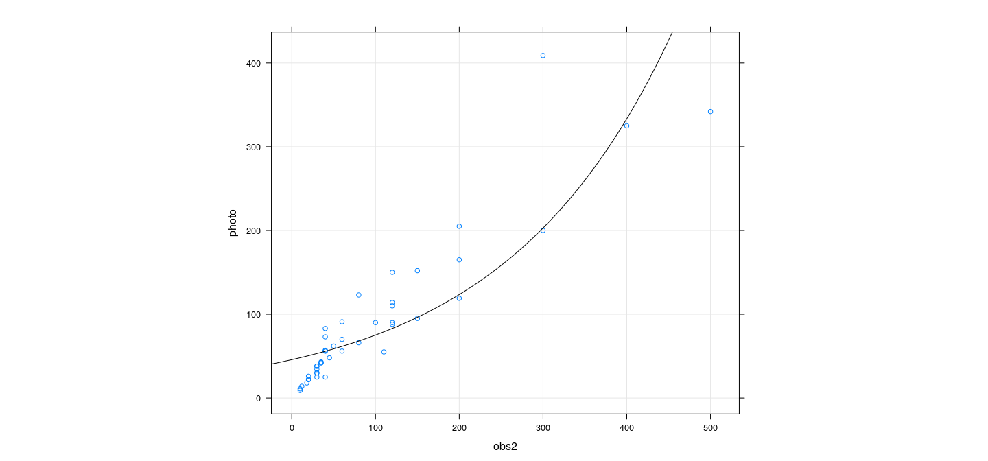
Example: Poisson response for snow geese flock counts
Call:
glm(formula = photo ~ obs2, family = poisson("identity"), data = snowgeese)

Deviance Residuals:
    Min       1Q   Median       3Q      Max
-5.0628  -1.6622  -0.3158   1.3064   8.6863

Coefficients:
            Estimate Std. Error z value Pr(>|z|)
(Intercept) 11.22312    1.39585    8.04 8.96e-16 ***
obs2         0.82102    0.01948   42.14  < 2e-16 ***
---
Signif. codes:  0 '***' 0.001 '**' 0.01 '*' 0.05 '.' 0.1 ' ' 1

(Dispersion parameter for poisson family taken to be 1)

    Null deviance: 2939.73  on 44  degrees of freedom
Residual deviance:  324.55  on 43  degrees of freedom
AIC: 596.51

Number of Fisher Scoring iterations: 6
Example: Poisson response for snow geese flock counts
xyplot(photo ~ obs2, snowgeese, grid = TRUE, aspect = "iso") +
    layer(panel.curve(predict(fmp3, newdata = list(obs2 = x), type = "response")))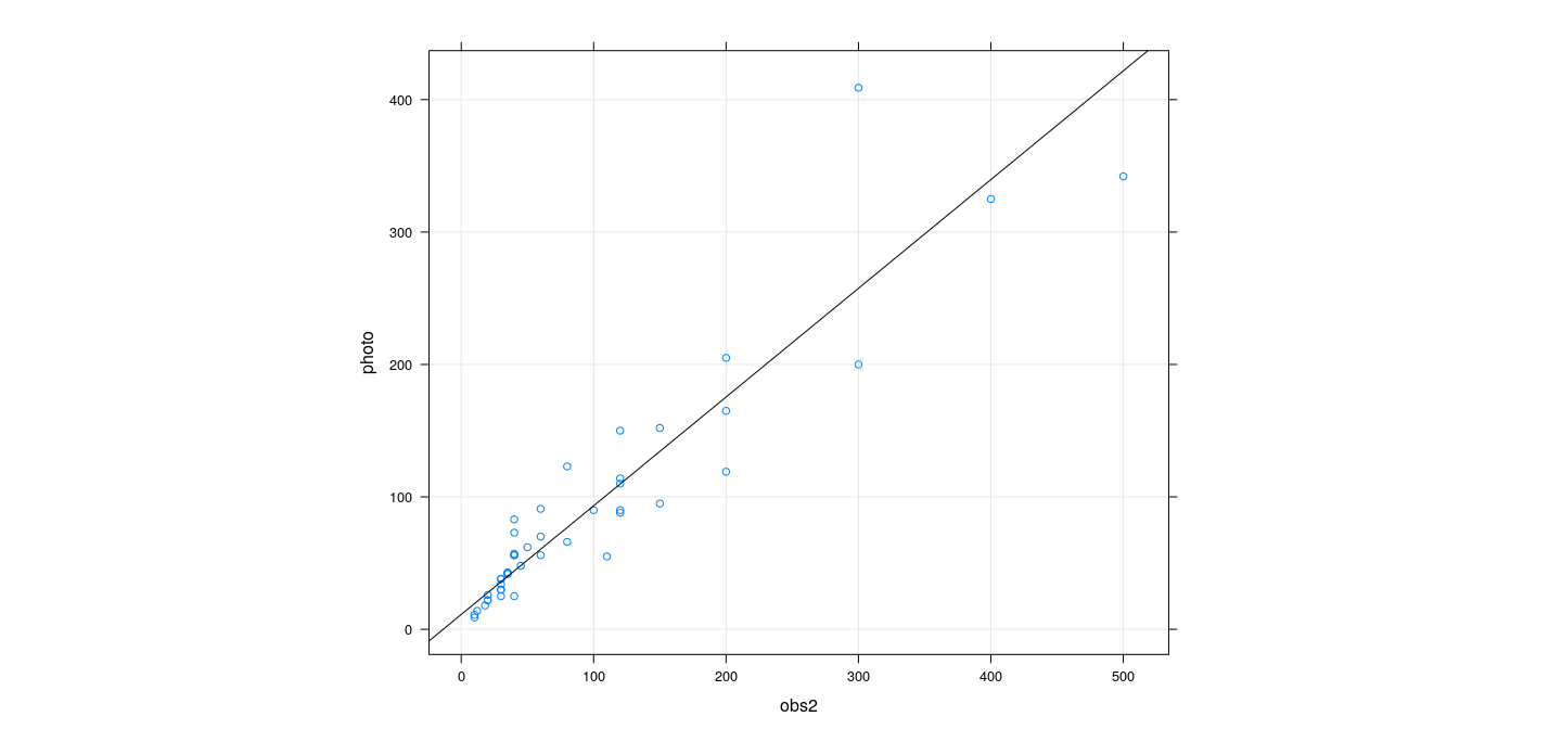
Diagnostics for GLMs
For the most part, based on (final) WLS approximation
Hat-values: Can be taken from WLS approximation (technically depends on \(y\) as well as \(X\))
Residuals: can be of several types,
residuals(object, type = ...)in R"response": \(y_i - \hat\mu_i\)"working": \(z_i - \hat\eta_i\) (residuals from WLS approximation)"deviance": square root of \(i\)-th component of deviance (with appropriate sign)"pearson": \(\frac{\sqrt{\hat\varphi} (y_i - \hat\mu_i)}{\sqrt{\hat{V}(y_i)}}\)
Other diagnostic measures and plots have similar generalizations
Quasi-likelihood families
Binomial and Poisson families have \(\varphi = 1\)
We can still pretend that there is a dispersion parameter \(\varphi\) during estimation
There is no corresponding response distribution or likelihood
The IRLS procedure still works (and gives identical estimates for \(\beta\))
However, estimated \(\hat\varphi > 1\) indicates overdispersion
Tests can be adjusted accordingly
This approach is known as quasi-likelihood estimation
Example: Quasi-Poisson model for snow geese counts
Call:
glm(formula = photo ~ obs2, family = quasipoisson("identity"),
    data = snowgeese)

Deviance Residuals:
    Min       1Q   Median       3Q      Max
-5.0628  -1.6622  -0.3158   1.3064   8.6863

Coefficients:
            Estimate Std. Error t value Pr(>|t|)
(Intercept) 11.22312    3.93720   2.851  0.00668 **
obs2         0.82102    0.05496  14.939  < 2e-16 ***
---
Signif. codes:  0 '***' 0.001 '**' 0.01 '*' 0.05 '.' 0.1 ' ' 1

(Dispersion parameter for quasipoisson family taken to be 7.956067)

    Null deviance: 2939.73  on 44  degrees of freedom
Residual deviance:  324.55  on 43  degrees of freedom
AIC: NA

Number of Fisher Scoring iterations: 6