Model Selection
Deepayan Sarkar
Model selection
Regression problems often have many predictors
The number of possible models increase rapidly with number of predictors
Even if we one of these models is “correct”, how do we find it?
Why does it matter?
One solution could be to use all the predictors
This is technically a valid model
Unfortunately this usually leads to unnecessarily high prediction error
Alternative: find “smallest” model for which \(F\)-test comparing to full model is accepted
This leads to multiple testing, inflated Type I error probability (and no obvious fix)
Model selection is usually based on some alternative criteria developed specifically for that purpose
Underfitting vs overfitting: the bias-variance trade-off
The basic problem in model selection is the familiar bias-variance trade-off problem
Underfitting leads to biased coefficient estimates
Overfitting leads to coefficient estimates with higher variance
Underfitting vs overfitting: the bias-variance trade-off
- Formally, suppose we fit the two models
If the second model is correct, then \(\hat{\beta}_1^{(1)}\) obtained by fitting the first model will be biased for \(\beta_1\) in general
If the first model is correct, then \(\hat{\beta}_1^{(2)}\) obtained by fitting the second model will be unbiased for \(\beta_1\)
However, in that case, \(\hat{\beta}_1^{(2)}\) will have higher variance than \(\hat{\beta}_1^{(1)}\) in general; i.e., for any vector \(\mathbf{u}\),
\[ V\left(\mathbf{u}^T \hat{\beta}_1^{(2)} \right) \geq V\left( \mathbf{u}^T \hat{\beta}_1^{(1)} \right) \]
- Proof: exercise
Model selection criteria
Overly simple and overly complex models are both bad
Best model usually lies somewhere in the middle
How do we find this ideal model?
Most common approach: some model-selection criterion measuring overall quality of a model
To be useful, such a criterion must punish both overly simple and overly complex models
Once criterion is determined, fit a number of different models and choose the best (details later)
We will first discuss some possible criteria
Coefficient of determination
- The simplest model quality measure is \(R^2\)
\[ R^{2}=\frac{T^{2}-S^{2}}{T^{2}} = \frac{\frac{T^{2}}{n}-\frac{S^{2}}{n}}{\frac{T^{2}}{n}} \]
Always increases when more predictors are added (does not penalize complexity)
Can compare models of same size, but not generally useful for model selection
Possible alternative: Adjusted \(R^{2}\) (substitute unbiased estimators of \(\sigma^2\))
\[ R_{adj}^{2}=\frac{\frac{T^{2}}{n-1}-\frac{S^{2}}{n-p}}{\frac{T^{2}}{n-1}}=1-\frac{n-1}{n-p}( 1-R^{2}) \]
Coefficient of determination
Maximizing \(R^2\) equivalent to minimizing SSE (or \(\hat{\sigma}^2_{MLE}\))
Maximizing \(R_{adj}^2\) equivalent to minimizing unbiased \(\hat{\sigma}^2\)
Other than simplicity of interpretation, no particular justification
Cross-validation SSE
Use cross-validation to directly assess prediction error
Define \[ T_{p}^{2}=\sum_{i=1}^n \left( y_{i} - \bar{y}_{(-i)}\right)^{2} \] and \[ S_{p}^{2} = \sum_{i=1}^n \left( y_{i}-\hat{y}_{i(-i)} \right)^{2} = \sum_{i=1}^n \left( \frac{e_i}{1-h_i} \right)^{2} \]
The predictive \(R^{2}\) is defined as \[ R_{p}^{2}=\frac{T_{p}^{2}-S_{p}^{2}}{T_{p}^{2}} \]
Equivalently, minimize predictive sum of squares \(S_{p}^{2}\) (often abbreviated as PRESS)
Directly estimating bias and variance
More sophisticated approaches attempt to directly estimate bias and variance
Suppose true expected value of \(y_i\) is \(\mu_i\)
Total mean squared error of a model fit is
\[ MSE = E \sum_i (\hat{y}_i - \mu_i)^2 = \sum_i \left[ (E\hat{y}_i - \mu_i)^2 + V(\hat{y}_i) \right] \]
The first term is the “bias sum of squares” \(BSS\) (equals zero if no bias)
The second term simplifies to
\[ \sum_i V(\hat{y}_i) = \sigma^2 \sum_i \mathbf{x}_i^T (\mathbf{X}^T \mathbf{X})^{-1} \mathbf{x}_i = \sigma^2 \sum_i h_i = p \sigma^2 \]
Directly estimating bias and variance
- On the other hand
\[ E(RSS) = E \sum_i ( y_i - \hat{y}_i)^2 = E (\mathbf{y}^T (\mathbf{I} - \mathbf{H}) \mathbf{y} ) \]
This equals \((n-p) \sigma^2\) when \(\hat{y}_i\)-s are unbiased
If \(\hat{y}_i\)-s are biased, it can be shown that this term equals \(BSS + (n-p) \sigma^2\)
This gives the following estimator of \(MSE\) (up to unknown \(\sigma^2\))
\[ RSS - (n-p) \sigma^2 + p \sigma^2 = RSS + (2p-n) \sigma^2 \]
Mallow’s \(C_p\)
- Dividing by \(\sigma^2\) on both sides, this gives Mallow’s \(C_p\) criterion
\[ C_p = \frac{RSS}{\sigma^2} + 2p - n \]
This requires an estimate of \(\sigma^2\)
It is customary to use \(\hat{\sigma}^2\) from the largest model
If model has no bias, then \(C_p \approx p\) (exact for largest model by definition)
An alternative expression for \(C_p\) is (exercise)
\[ C_p = (p_f - p) (F - 1) + p \]
- where
- \(p_f\) is the number of coefficients in the largest model (used to estimate \(\sigma^2\))
- \(F\) is the \(F\)-statistic comparing the model being evaluated with the largest model
- Again, if the model is “correct”, then \(F \approx 1\), so \(C_p \approx p\)
Likelihood based criterion
- A more general approach is to prefer models that improve the expected log-likelihood
\[ E \sum_i \log P_{\hat{\theta}}(y_i) \]
Here the expectation is over two independent sets of the true distribution of \(\mathbf{y}\)
One set of \(\mathbf{y}\) is used to estimate \(\hat\theta\)
Akaike showed that
\[ - 2E \sum_i \log P_{\hat{\theta}}(y_i) \approx -2 E (\text{loglik}) + 2p \]
- Here \(\text{loglik}\) is the maximized log-likelihood for the fitted model
Akaike Information Criterion
- This suggests the Akaike Information Criterion (AIC)
\[ \text{AIC} = -2 \text{loglik} + 2p \]
- For linear models, this is equivalent to (up to a constant)
\[ \text{AIC} = n \log RSS + 2p \]
An advantage of AIC over \(C_p\) is that it does not require an estimate of \(\sigma^2\)
It is also applicable more generally (e.g., for GLMs)
Bayesian Information Criterion
- A similar criterion is the Bayesian Information Criterion (BIC)
\[ \text{BIC} = -2 \text{loglik} + p \log n \]
As suggested by its name, this is derived using a Bayesian approach
The complexity penalty for BIC is higher (except for small \(n\)), so favours simpler models
Example: SLID data — comparing pre-determined set of models
SLID2 <- transform(na.omit(SLID), log.wages = log(wages), edu.sq = education^2)
SLID2 <- SLID2[c("log.wages", "sex", "edu.sq", "age", "language")]
str(SLID2)
'data.frame': 3987 obs. of 5 variables:
$ log.wages: num 2.36 2.4 2.88 2.64 2.1 ...
$ sex : Factor w/ 2 levels "Female","Male": 2 2 2 1 2 1 1 1 2 2 ...
$ edu.sq : num 225 174 196 256 225 ...
$ age : int 40 19 46 50 31 30 61 46 43 17 ...
$ language : Factor w/ 3 levels "English","French",..: 1 1 3 1 1 1 1 3 1 1 ...fm <- list()
fm[["S+E+A"]] <- lm(log.wages ~ sex + edu.sq + poly(age, 2), data = SLID2)
fm[["S+E+A+L"]] <- lm(log.wages ~ sex + edu.sq + poly(age, 2) + language, data = SLID2)
fm[["+ SE"]] <- update(fm[[2]], . ~ . + sex:edu.sq)
fm[["+ SA"]] <- update(fm[[2]], . ~ . + sex:poly(age, 2))
fm[["+ EA"]] <- update(fm[[2]], . ~ . + edu.sq:poly(age, 2))
fm[["(S+E+A)^2"]] <- update(fm[[2]], . ~ . + (sex + edu.sq + poly(age, 2))^2)
fm[["(S+E+A+L)^2"]] <- update(fm[[2]], . ~ . + (sex + edu.sq + poly(age, 2) + language)^2)
fm[["(S+E+A)^3"]] <- update(fm[[2]], . ~ . + (sex + edu.sq + poly(age, 2))^3)
fm[["(S+E+A+L)^3"]] <- update(fm[[2]], . ~ . + (sex + edu.sq + poly(age, 2) + language)^3)
models <- factor(names(fm), levels = names(fm))Example: SLID data — \(R^2\) and adjusted \(R^2\)
R2 <- sapply(fm, function(fit) summary(fit)$r.squared)
adj.R2 <- sapply(fm, function(fit) summary(fit)$adj.r.squared)
dotplot(R2 + adj.R2 ~ models, type = "o", pch = 16)
Example: SLID data — prediction SS
PRESS <- sapply(fm, function(fit) sum((residuals(fit) / (1-hatvalues(fit)))^2))
dotplot(PRESS ~ models, type = "o", pch = 16)
Example: SLID data — Mallow’s \(C_p\)
sigma.sq <- summary(fm[[9]])$sigma^2 # common 'scale' for all fits
Cp <- sapply(fm, function(fit) extractAIC(fit, scale = sigma.sq)[2])
dotplot(Cp ~ models, type = "o", pch = 16)
Example: SLID data — AIC
Example: SLID data — BIC
n <- nrow(SLID2)
BIC <- sapply(fm, function(fit) extractAIC(fit, k = log(n))[2])
dotplot(BIC ~ models, type = "o", pch = 16)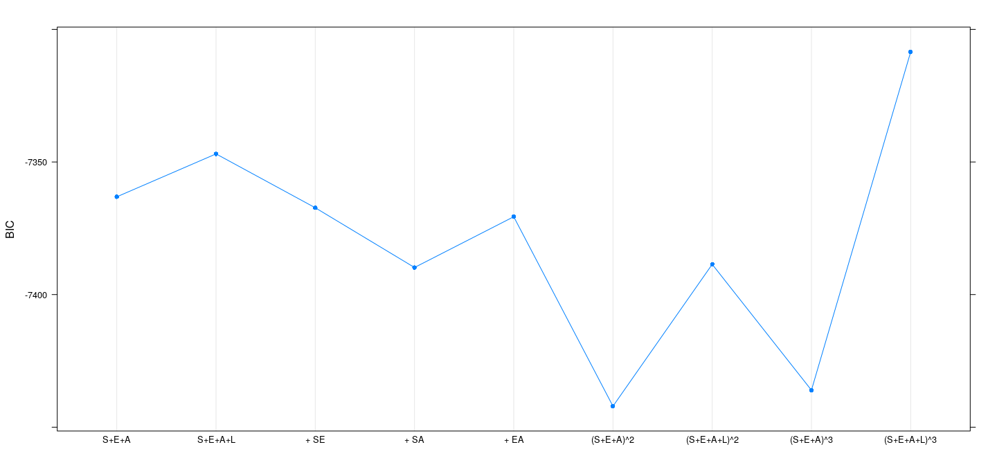
Automatic model selection
This process still requires us to construct a list of models to consider
In general, the number of possible models can be large
With \(k\) predictors, there are \(2^k\) additive models, many more with interactions
How do we select the “best” out of all possible models?
Two common strategies
- Best subset selection: exhaustive search of all possible models
- Stepwise selection: add or drop one term at a time (only benefit: needs less time)
Best subset selection: exhaustive search
library(leaps)
reg.sub <- regsubsets(log.wages ~ (sex + edu.sq + poly(age, 2) + language)^3,
                      data = SLID2, nbest = 2, nvmax = 100)
t(summary(reg.sub)$outmat)
1 ( 1 ) 1 ( 2 ) 2 ( 1 ) 2 ( 2 ) 3 ( 1 ) 3 ( 2 ) 4 ( 1 ) 4 ( 2 ) 5 ( 1 )
sexMale " " " " " " " " " " " " "*" "*" "*"
edu.sq " " " " " " " " " " "*" "*" "*" "*"
poly(age, 2)1 " " "*" " " " " " " "*" "*" "*" " "
poly(age, 2)2 " " " " " " "*" " " "*" "*" " " " "
languageFrench " " " " " " " " " " " " " " " " " "
languageOther " " " " " " " " " " " " " " " " " "
sexMale:edu.sq " " " " " " " " "*" " " " " " " " "
sexMale:poly(age, 2)1 " " " " " " " " " " " " " " " " "*"
sexMale:poly(age, 2)2 " " " " " " " " " " " " " " " " " "
sexMale:languageFrench " " " " " " " " " " " " " " " " " "
sexMale:languageOther " " " " " " " " " " " " " " " " " "
edu.sq:poly(age, 2)1 "*" " " "*" "*" "*" " " " " " " "*"
edu.sq:poly(age, 2)2 " " " " "*" " " "*" " " " " "*" "*"
edu.sq:languageFrench " " " " " " " " " " " " " " " " " "
edu.sq:languageOther " " " " " " " " " " " " " " " " " "
poly(age, 2)1:languageFrench " " " " " " " " " " " " " " " " " "
poly(age, 2)2:languageFrench " " " " " " " " " " " " " " " " " "
poly(age, 2)1:languageOther " " " " " " " " " " " " " " " " " "
poly(age, 2)2:languageOther " " " " " " " " " " " " " " " " " "
sexMale:edu.sq:poly(age, 2)1 " " " " " " " " " " " " " " " " " "
sexMale:edu.sq:poly(age, 2)2 " " " " " " " " " " " " " " " " " "
sexMale:edu.sq:languageFrench " " " " " " " " " " " " " " " " " "
sexMale:edu.sq:languageOther " " " " " " " " " " " " " " " " " "
sexMale:poly(age, 2)1:languageFrench " " " " " " " " " " " " " " " " " "
sexMale:poly(age, 2)2:languageFrench " " " " " " " " " " " " " " " " " "
sexMale:poly(age, 2)1:languageOther " " " " " " " " " " " " " " " " " "
sexMale:poly(age, 2)2:languageOther " " " " " " " " " " " " " " " " " "
edu.sq:poly(age, 2)1:languageFrench " " " " " " " " " " " " " " " " " "
edu.sq:poly(age, 2)2:languageFrench " " " " " " " " " " " " " " " " " "
edu.sq:poly(age, 2)1:languageOther " " " " " " " " " " " " " " " " " "
edu.sq:poly(age, 2)2:languageOther " " " " " " " " " " " " " " " " " "
5 ( 2 ) 6 ( 1 ) 6 ( 2 ) 7 ( 1 ) 7 ( 2 ) 8 ( 1 ) 8 ( 2 ) 9 ( 1 ) 9 ( 2 )
sexMale "*" "*" "*" "*" "*" "*" "*" "*" "*"
edu.sq "*" "*" "*" "*" "*" "*" "*" "*" "*"
poly(age, 2)1 "*" " " " " " " " " " " "*" " " " "
poly(age, 2)2 "*" "*" " " " " "*" " " " " " " "*"
languageFrench " " " " " " " " " " " " " " " " " "
languageOther " " " " " " " " " " " " " " " " " "
sexMale:edu.sq " " " " "*" "*" "*" "*" "*" "*" "*"
sexMale:poly(age, 2)1 "*" "*" "*" "*" "*" "*" "*" "*" "*"
sexMale:poly(age, 2)2 " " " " " " "*" " " "*" "*" "*" "*"
sexMale:languageFrench " " " " " " " " " " " " " " " " " "
sexMale:languageOther " " " " " " " " " " " " " " " " " "
edu.sq:poly(age, 2)1 " " "*" "*" "*" "*" "*" "*" "*" "*"
edu.sq:poly(age, 2)2 " " " " "*" "*" " " "*" "*" "*" "*"
edu.sq:languageFrench " " " " " " " " " " " " " " " " " "
edu.sq:languageOther " " " " " " " " " " " " " " " " " "
poly(age, 2)1:languageFrench " " " " " " " " " " " " " " " " " "
poly(age, 2)2:languageFrench " " " " " " " " " " " " " " " " " "
poly(age, 2)1:languageOther " " " " " " " " " " " " " " " " " "
poly(age, 2)2:languageOther " " " " " " " " " " " " " " " " " "
sexMale:edu.sq:poly(age, 2)1 " " "*" " " " " "*" "*" " " "*" "*"
sexMale:edu.sq:poly(age, 2)2 " " " " " " " " " " " " " " "*" " "
sexMale:edu.sq:languageFrench " " " " " " " " " " " " " " " " " "
sexMale:edu.sq:languageOther " " " " " " " " " " " " " " " " " "
sexMale:poly(age, 2)1:languageFrench " " " " " " " " " " " " " " " " " "
sexMale:poly(age, 2)2:languageFrench " " " " " " " " " " " " " " " " " "
sexMale:poly(age, 2)1:languageOther " " " " " " " " " " " " " " " " " "
sexMale:poly(age, 2)2:languageOther " " " " " " " " " " " " " " " " " "
edu.sq:poly(age, 2)1:languageFrench " " " " " " " " " " " " " " " " " "
edu.sq:poly(age, 2)2:languageFrench " " " " " " " " " " " " " " " " " "
edu.sq:poly(age, 2)1:languageOther " " " " " " " " " " " " " " " " " "
edu.sq:poly(age, 2)2:languageOther " " " " " " " " " " " " " " " " " "
10 ( 1 ) 10 ( 2 ) 11 ( 1 ) 11 ( 2 ) 12 ( 1 ) 12 ( 2 ) 13 ( 1 ) 13 ( 2 )
sexMale "*" "*" "*" "*" "*" "*" "*" "*"
edu.sq "*" "*" "*" "*" "*" "*" "*" "*"
poly(age, 2)1 " " " " " " " " "*" "*" "*" "*"
poly(age, 2)2 " " " " " " " " " " " " " " " "
languageFrench " " " " " " " " " " " " " " " "
languageOther " " " " " " " " " " " " " " " "
sexMale:edu.sq "*" "*" "*" "*" "*" "*" "*" "*"
sexMale:poly(age, 2)1 "*" "*" "*" "*" "*" "*" "*" "*"
sexMale:poly(age, 2)2 "*" "*" "*" "*" "*" "*" "*" "*"
sexMale:languageFrench " " " " " " " " " " " " " " " "
sexMale:languageOther " " " " " " " " " " " " " " "*"
edu.sq:poly(age, 2)1 "*" "*" "*" "*" "*" "*" "*" "*"
edu.sq:poly(age, 2)2 "*" "*" "*" "*" "*" "*" "*" "*"
edu.sq:languageFrench " " " " " " " " " " " " " " " "
edu.sq:languageOther " " " " " " " " " " " " " " " "
poly(age, 2)1:languageFrench " " " " " " " " " " " " " " " "
poly(age, 2)2:languageFrench " " " " " " " " " " " " " " " "
poly(age, 2)1:languageOther " " " " " " " " " " " " " " " "
poly(age, 2)2:languageOther " " "*" " " " " " " " " " " " "
sexMale:edu.sq:poly(age, 2)1 "*" "*" "*" "*" "*" "*" "*" "*"
sexMale:edu.sq:poly(age, 2)2 "*" "*" "*" "*" "*" "*" "*" "*"
sexMale:edu.sq:languageFrench " " " " " " " " " " " " "*" " "
sexMale:edu.sq:languageOther " " " " " " " " " " " " " " " "
sexMale:poly(age, 2)1:languageFrench " " " " " " "*" " " "*" " " " "
sexMale:poly(age, 2)2:languageFrench " " " " " " " " " " " " " " " "
sexMale:poly(age, 2)1:languageOther " " " " " " " " " " " " " " " "
sexMale:poly(age, 2)2:languageOther "*" " " "*" "*" "*" "*" "*" "*"
edu.sq:poly(age, 2)1:languageFrench " " " " "*" " " "*" " " "*" "*"
edu.sq:poly(age, 2)2:languageFrench " " " " " " " " " " " " " " " "
edu.sq:poly(age, 2)1:languageOther " " " " " " " " " " " " " " " "
edu.sq:poly(age, 2)2:languageOther " " " " " " " " " " " " " " " "
14 ( 1 ) 14 ( 2 ) 15 ( 1 ) 15 ( 2 ) 16 ( 1 ) 16 ( 2 ) 17 ( 1 ) 17 ( 2 )
sexMale "*" "*" "*" "*" "*" "*" "*" "*"
edu.sq "*" "*" "*" "*" "*" "*" "*" "*"
poly(age, 2)1 "*" "*" "*" "*" "*" "*" "*" "*"
poly(age, 2)2 " " " " "*" "*" "*" "*" "*" "*"
languageFrench " " " " " " " " " " " " " " " "
languageOther " " " " " " " " " " " " " " " "
sexMale:edu.sq "*" "*" "*" "*" "*" "*" "*" "*"
sexMale:poly(age, 2)1 "*" "*" "*" "*" "*" "*" "*" "*"
sexMale:poly(age, 2)2 "*" "*" "*" "*" "*" "*" "*" "*"
sexMale:languageFrench " " " " " " " " " " "*" "*" " "
sexMale:languageOther "*" "*" "*" "*" "*" "*" "*" "*"
edu.sq:poly(age, 2)1 "*" "*" "*" "*" "*" "*" "*" "*"
edu.sq:poly(age, 2)2 "*" "*" "*" "*" "*" "*" "*" "*"
edu.sq:languageFrench " " " " " " " " " " " " " " " "
edu.sq:languageOther " " " " " " " " " " " " " " "*"
poly(age, 2)1:languageFrench " " " " " " " " " " " " " " " "
poly(age, 2)2:languageFrench " " " " " " " " " " " " " " " "
poly(age, 2)1:languageOther " " " " " " " " " " " " " " " "
poly(age, 2)2:languageOther " " " " " " " " " " " " " " " "
sexMale:edu.sq:poly(age, 2)1 "*" "*" "*" "*" "*" "*" "*" "*"
sexMale:edu.sq:poly(age, 2)2 "*" "*" "*" "*" "*" "*" "*" "*"
sexMale:edu.sq:languageFrench "*" "*" "*" "*" "*" "*" "*" "*"
sexMale:edu.sq:languageOther " " " " " " " " " " " " " " " "
sexMale:poly(age, 2)1:languageFrench " " "*" " " "*" " " "*" "*" " "
sexMale:poly(age, 2)2:languageFrench " " " " " " " " " " " " " " " "
sexMale:poly(age, 2)1:languageOther " " " " " " " " "*" " " "*" "*"
sexMale:poly(age, 2)2:languageOther "*" "*" "*" "*" "*" "*" "*" "*"
edu.sq:poly(age, 2)1:languageFrench "*" " " "*" " " "*" " " " " "*"
edu.sq:poly(age, 2)2:languageFrench " " " " " " " " " " " " " " " "
edu.sq:poly(age, 2)1:languageOther " " " " " " " " " " " " " " " "
edu.sq:poly(age, 2)2:languageOther " " " " " " " " " " " " " " " "
18 ( 1 ) 18 ( 2 ) 19 ( 1 ) 19 ( 2 ) 20 ( 1 ) 20 ( 2 ) 21 ( 1 ) 21 ( 2 )
sexMale "*" "*" "*" "*" "*" "*" "*" "*"
edu.sq "*" "*" "*" "*" "*" "*" "*" "*"
poly(age, 2)1 "*" "*" "*" "*" "*" "*" "*" "*"
poly(age, 2)2 "*" "*" "*" "*" "*" "*" "*" "*"
languageFrench " " "*" " " " " " " "*" " " "*"
languageOther " " " " " " " " " " " " " " " "
sexMale:edu.sq "*" "*" "*" "*" "*" "*" "*" "*"
sexMale:poly(age, 2)1 "*" "*" "*" "*" "*" "*" "*" "*"
sexMale:poly(age, 2)2 "*" "*" "*" "*" "*" "*" "*" "*"
sexMale:languageFrench "*" " " "*" "*" "*" " " "*" " "
sexMale:languageOther "*" "*" "*" "*" "*" "*" "*" "*"
edu.sq:poly(age, 2)1 "*" "*" "*" "*" "*" "*" "*" "*"
edu.sq:poly(age, 2)2 "*" "*" "*" "*" "*" "*" "*" "*"
edu.sq:languageFrench " " " " " " "*" " " " " " " " "
edu.sq:languageOther "*" "*" "*" "*" "*" "*" "*" "*"
poly(age, 2)1:languageFrench " " " " " " " " " " " " " " " "
poly(age, 2)2:languageFrench " " " " " " " " " " " " " " " "
poly(age, 2)1:languageOther " " " " " " " " " " " " "*" "*"
poly(age, 2)2:languageOther " " " " " " " " " " " " " " " "
sexMale:edu.sq:poly(age, 2)1 "*" "*" "*" "*" "*" "*" "*" "*"
sexMale:edu.sq:poly(age, 2)2 "*" "*" "*" "*" "*" "*" "*" "*"
sexMale:edu.sq:languageFrench "*" "*" "*" "*" "*" "*" "*" "*"
sexMale:edu.sq:languageOther " " " " " " " " " " " " " " " "
sexMale:poly(age, 2)1:languageFrench "*" "*" "*" "*" "*" "*" "*" "*"
sexMale:poly(age, 2)2:languageFrench " " " " " " " " " " " " " " " "
sexMale:poly(age, 2)1:languageOther "*" "*" "*" "*" "*" "*" "*" "*"
sexMale:poly(age, 2)2:languageOther "*" "*" "*" "*" "*" "*" "*" "*"
edu.sq:poly(age, 2)1:languageFrench " " " " " " " " "*" "*" "*" "*"
edu.sq:poly(age, 2)2:languageFrench " " " " " " " " " " " " " " " "
edu.sq:poly(age, 2)1:languageOther " " " " "*" " " "*" "*" "*" "*"
edu.sq:poly(age, 2)2:languageOther " " " " " " " " " " " " " " " "
22 ( 1 ) 22 ( 2 ) 23 ( 1 ) 23 ( 2 ) 24 ( 1 ) 24 ( 2 ) 25 ( 1 ) 25 ( 2 )
sexMale "*" "*" "*" "*" "*" "*" "*" "*"
edu.sq "*" "*" "*" "*" "*" "*" "*" "*"
poly(age, 2)1 "*" "*" "*" "*" "*" "*" "*" "*"
poly(age, 2)2 "*" "*" "*" "*" "*" "*" "*" "*"
languageFrench "*" " " "*" " " " " "*" " " " "
languageOther " " " " " " " " " " " " " " " "
sexMale:edu.sq "*" "*" "*" "*" "*" "*" "*" "*"
sexMale:poly(age, 2)1 "*" "*" "*" "*" "*" "*" "*" "*"
sexMale:poly(age, 2)2 "*" "*" "*" "*" "*" "*" "*" "*"
sexMale:languageFrench " " "*" " " "*" "*" "*" "*" "*"
sexMale:languageOther "*" "*" "*" "*" "*" "*" "*" "*"
edu.sq:poly(age, 2)1 "*" "*" "*" "*" "*" "*" "*" "*"
edu.sq:poly(age, 2)2 "*" "*" "*" "*" "*" "*" "*" "*"
edu.sq:languageFrench " " " " " " "*" "*" " " "*" "*"
edu.sq:languageOther "*" "*" "*" "*" "*" "*" "*" "*"
poly(age, 2)1:languageFrench "*" "*" "*" "*" "*" "*" "*" "*"
poly(age, 2)2:languageFrench " " " " " " " " " " " " "*" " "
poly(age, 2)1:languageOther "*" "*" "*" "*" "*" "*" "*" "*"
poly(age, 2)2:languageOther " " " " " " " " " " " " " " " "
sexMale:edu.sq:poly(age, 2)1 "*" "*" "*" "*" "*" "*" "*" "*"
sexMale:edu.sq:poly(age, 2)2 "*" "*" "*" "*" "*" "*" "*" "*"
sexMale:edu.sq:languageFrench "*" "*" "*" "*" "*" "*" "*" "*"
sexMale:edu.sq:languageOther " " " " "*" " " "*" "*" "*" "*"
sexMale:poly(age, 2)1:languageFrench "*" "*" "*" "*" "*" "*" "*" "*"
sexMale:poly(age, 2)2:languageFrench " " " " " " " " " " " " " " " "
sexMale:poly(age, 2)1:languageOther "*" "*" "*" "*" "*" "*" "*" "*"
sexMale:poly(age, 2)2:languageOther "*" "*" "*" "*" "*" "*" "*" "*"
edu.sq:poly(age, 2)1:languageFrench "*" "*" "*" "*" "*" "*" "*" "*"
edu.sq:poly(age, 2)2:languageFrench " " " " " " " " " " " " " " " "
edu.sq:poly(age, 2)1:languageOther "*" "*" "*" "*" "*" "*" "*" "*"
edu.sq:poly(age, 2)2:languageOther " " " " " " " " " " " " " " "*"
26 ( 1 ) 26 ( 2 ) 27 ( 1 ) 27 ( 2 ) 28 ( 1 ) 28 ( 2 ) 29 ( 1 ) 29 ( 2 )
sexMale "*" "*" "*" "*" "*" "*" "*" "*"
edu.sq "*" "*" "*" "*" "*" "*" "*" "*"
poly(age, 2)1 "*" "*" "*" "*" "*" "*" "*" "*"
poly(age, 2)2 "*" "*" "*" "*" "*" "*" "*" "*"
languageFrench " " " " " " " " " " "*" "*" " "
languageOther " " " " " " " " " " " " " " "*"
sexMale:edu.sq "*" "*" "*" "*" "*" "*" "*" "*"
sexMale:poly(age, 2)1 "*" "*" "*" "*" "*" "*" "*" "*"
sexMale:poly(age, 2)2 "*" "*" "*" "*" "*" "*" "*" "*"
sexMale:languageFrench "*" "*" "*" "*" "*" "*" "*" "*"
sexMale:languageOther "*" "*" "*" "*" "*" "*" "*" "*"
edu.sq:poly(age, 2)1 "*" "*" "*" "*" "*" "*" "*" "*"
edu.sq:poly(age, 2)2 "*" "*" "*" "*" "*" "*" "*" "*"
edu.sq:languageFrench "*" "*" "*" "*" "*" "*" "*" "*"
edu.sq:languageOther "*" "*" "*" "*" "*" "*" "*" "*"
poly(age, 2)1:languageFrench "*" "*" "*" "*" "*" "*" "*" "*"
poly(age, 2)2:languageFrench "*" " " "*" "*" "*" "*" "*" "*"
poly(age, 2)1:languageOther "*" "*" "*" "*" "*" "*" "*" "*"
poly(age, 2)2:languageOther " " " " "*" " " "*" "*" "*" "*"
sexMale:edu.sq:poly(age, 2)1 "*" "*" "*" "*" "*" "*" "*" "*"
sexMale:edu.sq:poly(age, 2)2 "*" "*" "*" "*" "*" "*" "*" "*"
sexMale:edu.sq:languageFrench "*" "*" "*" "*" "*" "*" "*" "*"
sexMale:edu.sq:languageOther "*" "*" "*" "*" "*" "*" "*" "*"
sexMale:poly(age, 2)1:languageFrench "*" "*" "*" "*" "*" "*" "*" "*"
sexMale:poly(age, 2)2:languageFrench " " " " " " " " " " " " " " " "
sexMale:poly(age, 2)1:languageOther "*" "*" "*" "*" "*" "*" "*" "*"
sexMale:poly(age, 2)2:languageOther "*" "*" "*" "*" "*" "*" "*" "*"
edu.sq:poly(age, 2)1:languageFrench "*" "*" "*" "*" "*" "*" "*" "*"
edu.sq:poly(age, 2)2:languageFrench " " "*" " " "*" "*" " " "*" "*"
edu.sq:poly(age, 2)1:languageOther "*" "*" "*" "*" "*" "*" "*" "*"
edu.sq:poly(age, 2)2:languageOther "*" "*" "*" "*" "*" "*" "*" "*"
30 ( 1 ) 30 ( 2 ) 31 ( 1 )
sexMale "*" "*" "*"
edu.sq "*" "*" "*"
poly(age, 2)1 "*" "*" "*"
poly(age, 2)2 "*" "*" "*"
languageFrench "*" "*" "*"
languageOther " " "*" "*"
sexMale:edu.sq "*" "*" "*"
sexMale:poly(age, 2)1 "*" "*" "*"
sexMale:poly(age, 2)2 "*" "*" "*"
sexMale:languageFrench "*" "*" "*"
sexMale:languageOther "*" "*" "*"
edu.sq:poly(age, 2)1 "*" "*" "*"
edu.sq:poly(age, 2)2 "*" "*" "*"
edu.sq:languageFrench "*" "*" "*"
edu.sq:languageOther "*" "*" "*"
poly(age, 2)1:languageFrench "*" "*" "*"
poly(age, 2)2:languageFrench "*" "*" "*"
poly(age, 2)1:languageOther "*" "*" "*"
poly(age, 2)2:languageOther "*" "*" "*"
sexMale:edu.sq:poly(age, 2)1 "*" "*" "*"
sexMale:edu.sq:poly(age, 2)2 "*" "*" "*"
sexMale:edu.sq:languageFrench "*" "*" "*"
sexMale:edu.sq:languageOther "*" "*" "*"
sexMale:poly(age, 2)1:languageFrench "*" "*" "*"
sexMale:poly(age, 2)2:languageFrench "*" " " "*"
sexMale:poly(age, 2)1:languageOther "*" "*" "*"
sexMale:poly(age, 2)2:languageOther "*" "*" "*"
edu.sq:poly(age, 2)1:languageFrench "*" "*" "*"
edu.sq:poly(age, 2)2:languageFrench "*" "*" "*"
edu.sq:poly(age, 2)1:languageOther "*" "*" "*"
edu.sq:poly(age, 2)2:languageOther "*" "*" "*" Best subset selection: exhaustive search
xyplot(scale(bic) + scale(cp) ~ seq_along(bic), data = summary(reg.sub), grid = TRUE,
       type = "o", pch = 16)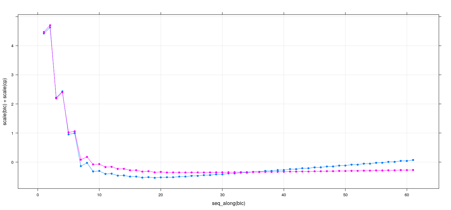
Best subset selection: exhaustive search
xyplot(scale(bic) + scale(cp) ~ seq_along(bic), data = summary(reg.sub), grid = TRUE,
       type = "o", pch = 16, ylim = c(NA, 0.5))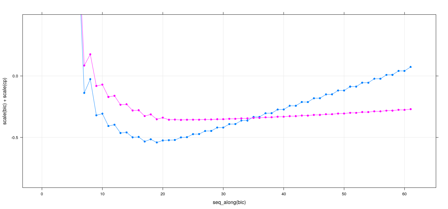
Best subset selection: exhaustive search
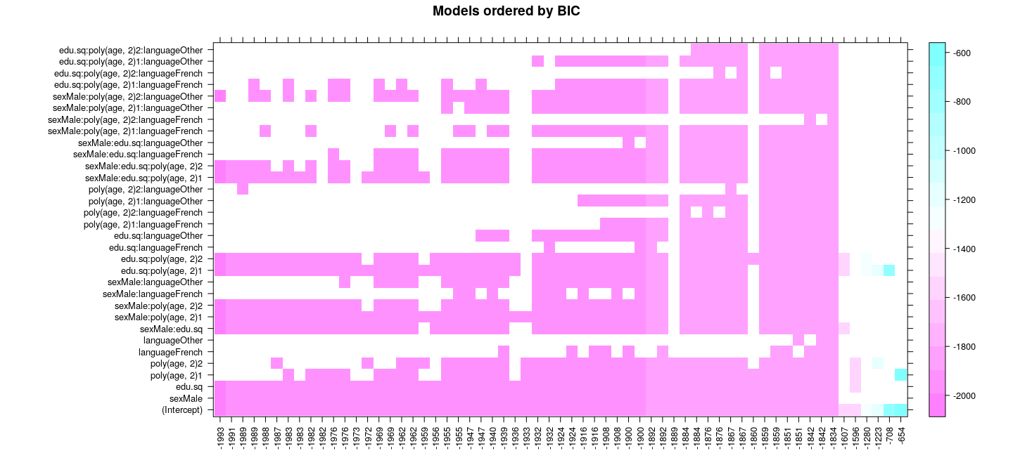
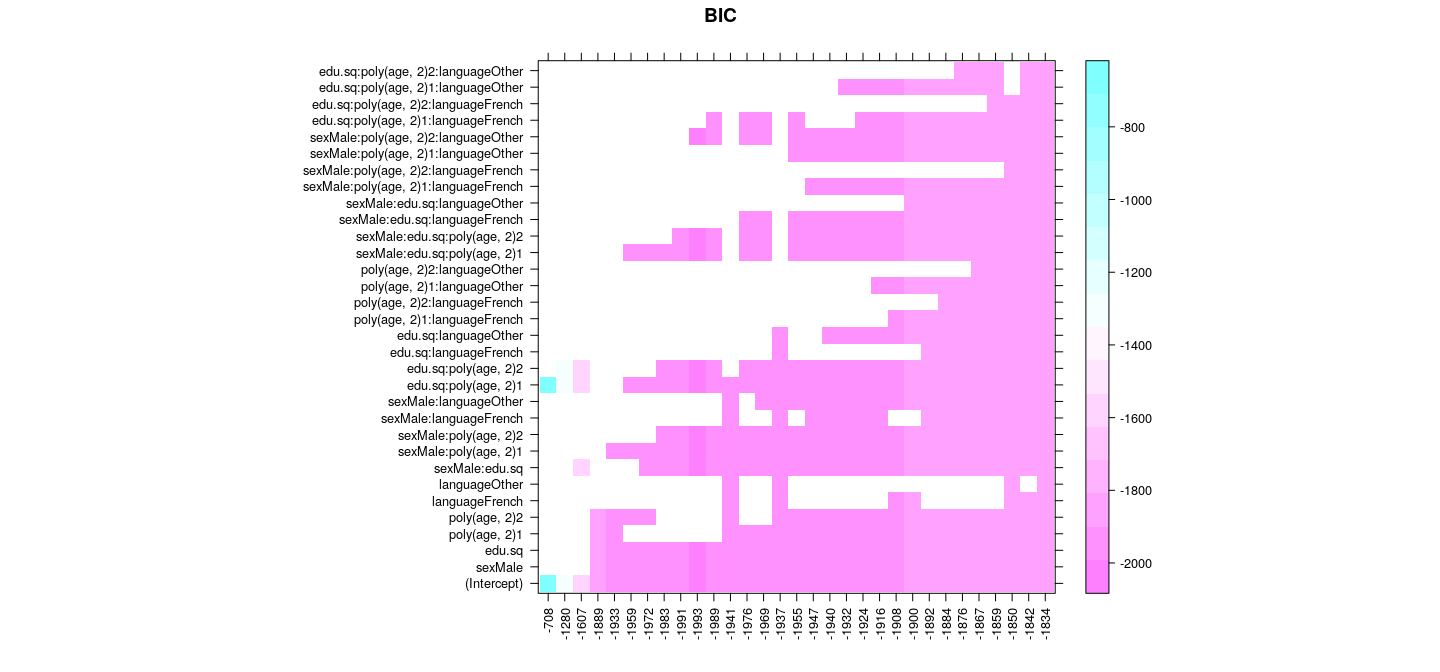
with(summary(reg.sub), {
         o <- order(bic); w <- which; is.na(w) <- w == FALSE
         wbic <- w * bic
         levelplot(wbic[o, ], xlim = as.character(round(bic))[o], xlab = NULL, ylab = NULL,
                   scales = list(x = list(rot = 90)), main = "Models ordered by BIC")
     })
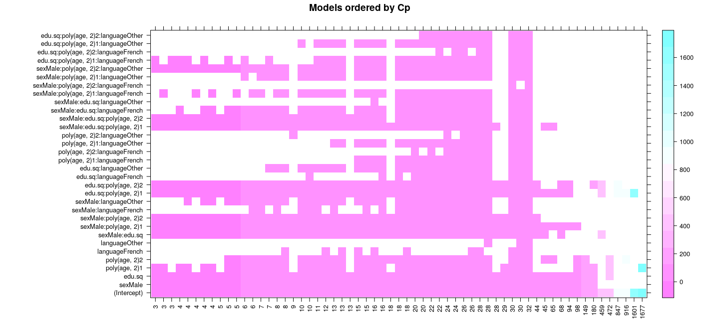
Best subset selection: exhaustive search
with(summary(reg.sub), {
         o <- order(cp); w <- which; is.na(w) <- w == FALSE
         wcp <- w * cp
         levelplot(wcp[o, ], xlim = as.character(round(cp))[o], xlab = NULL, ylab = NULL,
                   scales = list(x = list(rot = 90)), main = "Models ordered by Cp")
     })
Handling dummy variables, interactions, etc.
One problem with this approach: considers each column of \(\mathbf{X}\) separately
Usually we would keep or drop all columns for a term (factor, polynomial) together
Similarly, an interaction term usually not meaningful without main effects and lower order interactions
Such considerations are not automated by
regsubsets()and have to be handled manually
Best subset selection: stepwise search
Stepwise selection methods are greedy algorithms that add or drop one predtctor at a time
This greatly limits the number of subsets evaluated
Makes the problem tractable if number of predictors is large
On the other hand, stepwise methods explore only a fraction of possible subsets
For many predictors, rarely finds the optimal model
Best subset selection: stepwise search
- Forward selection
- Find best one-variable model
- Find best two-variable model by adding another variable
- and so on
That is, do not look at all two-variable models; only ones that contain the best one-variable model
Backward selection: start with full model and eliminate variables successively
Sequential replacement: consider both adding and dropping in each step
Stepwise selection is supported by
regsubsets()Also implemented in
MASS::stepAIC()andstats::step()
Best subset selection: forward selection
reg.forward <-
    regsubsets(log.wages ~ (sex + edu.sq + poly(age, 2) + language)^3,
               data = SLID2, nvmax = 100, method = "forward")
xyplot(bic ~ seq_along(bic), data = summary(reg.forward), grid = TRUE, type = "o", pch = 16)
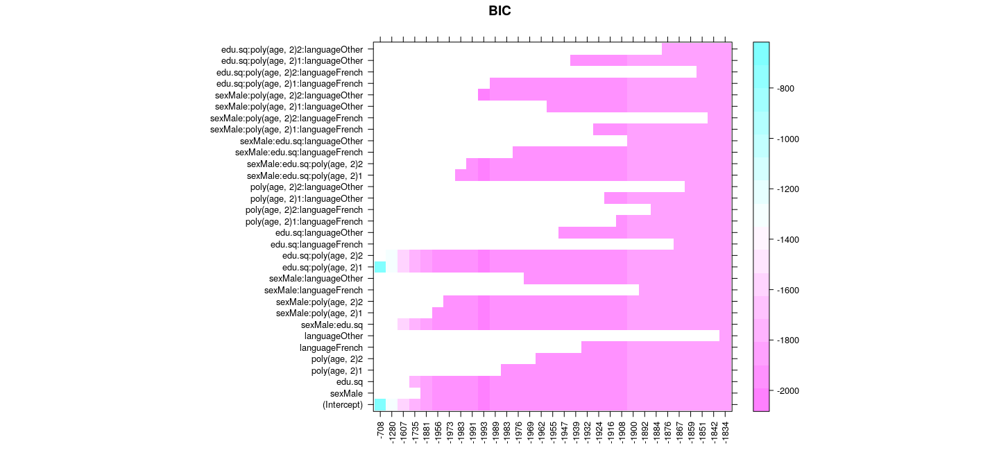
Best subset selection: forward selection
with(summary(reg.forward), {
         w <- which; is.na(w) <- w == FALSE
         wbic <- w * bic
         levelplot(wbic, xlim = as.character(round(bic)), xlab = NULL, ylab = NULL,
                   scales = list(x = list(rot = 90)), main = "BIC")
     })
Best subset selection: sequential replacement
reg.seqrep <-
    regsubsets(log.wages ~ (sex + edu.sq + poly(age, 2) + language)^3,
               data = SLID2, nvmax = 100, method = "seqrep")
xyplot(bic ~ seq_along(bic), data = summary(reg.seqrep), grid = TRUE, type = "o", pch = 16)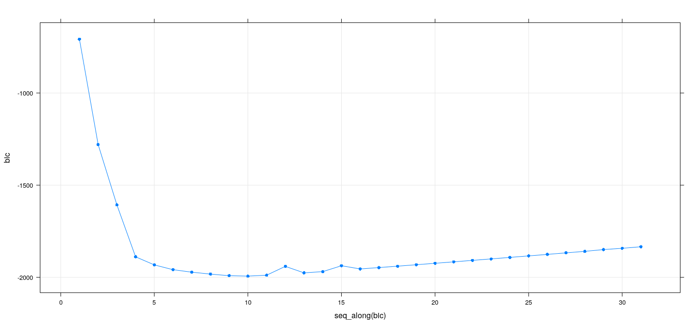
Best subset selection: sequential replacement
with(summary(reg.seqrep), {
         w <- which; is.na(w) <- w == FALSE
         wbic <- w * bic
         levelplot(wbic, xlim = as.character(round(bic)), xlab = NULL, ylab = NULL,
                   scales = list(x = list(rot = 90)), main = "BIC")
     })
Benefits and drawbacks of automated model selection
Can quickly survey a large number of potential models
However, there are many drawbacks to this approach
In fact, automated model selection basically invalidates inference
This is because all derivations assume that model and hypotheses are prespecified
As a result, for the model chosen by automated selection
Test statistics no longer follow \(t\) / \(F\) distributions
Standard errors have negative bias, and confidence intervals are falsely narrow
\(p\)-values are falsely small
Regression coefficients are biased away from 0
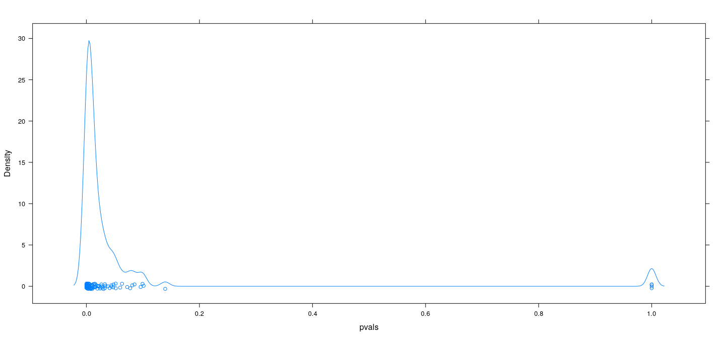
Simulation example: no predictive relationship
Simulate \(V_2, \dots, V_{21} \sim \text{ i.i.d. } N(0, 1)\)
Simulate independent \(V_1 \sim N(0, 1)\)
Regress \(V_1\) on \(V_2, \dots, V_{21}\)
Select model using
stepAIC()
Simulation example: no predictive relationship
Call:
lm(formula = V1 ~ V2 + V3 + V6 + V9 + V13, data = d)

Residuals:
     Min       1Q   Median       3Q      Max
-2.20598 -0.59320 -0.05848  0.56056  2.34801

Coefficients:
            Estimate Std. Error t value Pr(>|t|)
(Intercept) -0.03006    0.08906  -0.338  0.73645
V2           0.13104    0.09139   1.434  0.15493
V3          -0.16376    0.08943  -1.831  0.07026 .
V6          -0.29802    0.10074  -2.958  0.00391 **
V9           0.15936    0.08864   1.798  0.07542 .
V13          0.17006    0.08214   2.070  0.04116 *
---
Signif. codes:  0 '***' 0.001 '**' 0.01 '*' 0.05 '.' 0.1 ' ' 1

Residual standard error: 0.8665 on 94 degrees of freedom
Multiple R-squared:  0.1932,    Adjusted R-squared:  0.1503
F-statistic: 4.501 on 5 and 94 DF, p-value: 0.001011 value
0.00101054 Simulation example: no predictive relationship
## Replicate this experiment
pvals <-
    replicate(100,
    {
        d <- as.data.frame(matrix(rnorm(100 * 21), 100, 21))
        fm.step <- stepAIC(lm(V1 ~ ., data = d), direction = "both", trace = 0)
        if (length(coef(fm.step)) > 1)
            with(summary(fm.step), pf(fstatistic[1], fstatistic[2], fstatistic[3], lower.tail = FALSE))
        else 1
    })
sum(pvals < 0.05)
[1] 84Simulation example: no predictive relationship
Simulation example: no predictive relationship
Results are slightly better when using BIC rather than AIC, but still bad
Select model using
stepAIC(..., k = log(n))
pvals <-
    replicate(100,
    {
        d <- as.data.frame(matrix(rnorm(100 * 21), 100, 21))
        fm.step <- stepAIC(lm(V1 ~ ., data = d), direction = "both", trace = 0, k = log(100))
        if (length(coef(fm.step)) > 1)
            with(summary(fm.step), pf(fstatistic[1], fstatistic[2], fstatistic[3], lower.tail = FALSE))
        else 1
    })
sum(pvals < 0.05)
[1] 56Simulation example: no predictive relationship
Summary
Automated model selection has its uses
However, blindly applying it without thinking about the problem is dangerous
Many applied studies have no prespecified hypothesis
Especially in observational studies (e.g., public health and social sciences)
Model is often chosen by automated selection, but interpreted as if prespecified
Result: much more than 5% of “significant” results are probably false