Introduction to Nonparametric Regression
Deepayan Sarkar
Visualizing distributions
Recall that the goal of regression is to predict distribution of \(\mathbf{Y} | \mathbf{X=x}\)
How can we assess distribution visually? (e.g., to check normality)
Usual tools
- Histograms / density plots
- Box-and-whisker plots
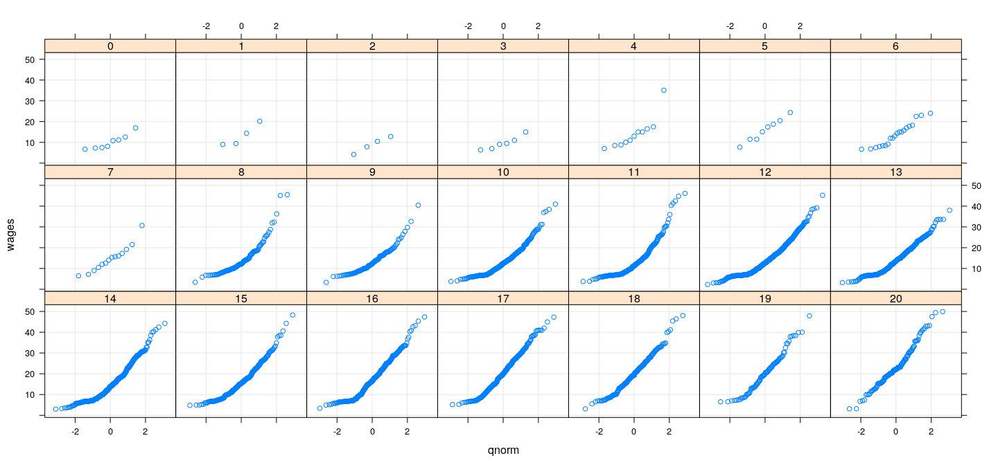
- Quantile-quantile plots
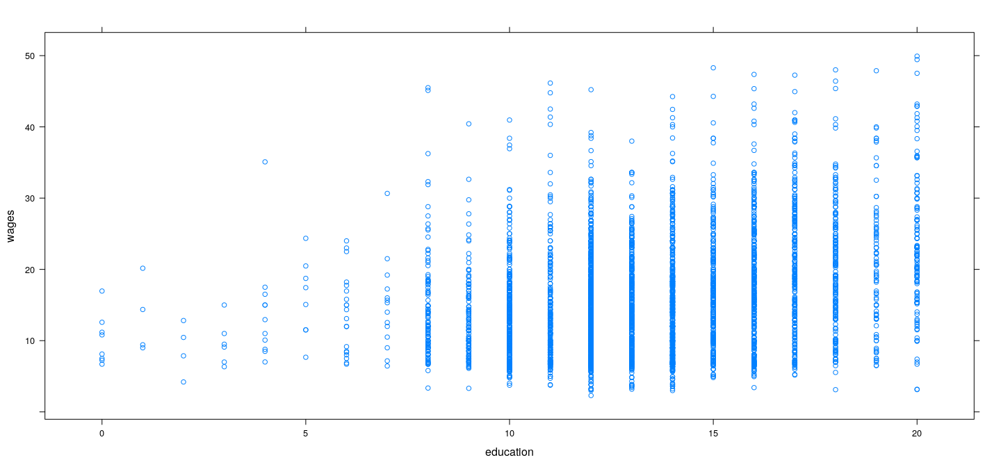
Example: SLID data
![plot of chunk unnamed-chunk-1]()
Example: SLID data (rounding education)
![plot of chunk unnamed-chunk-2]()
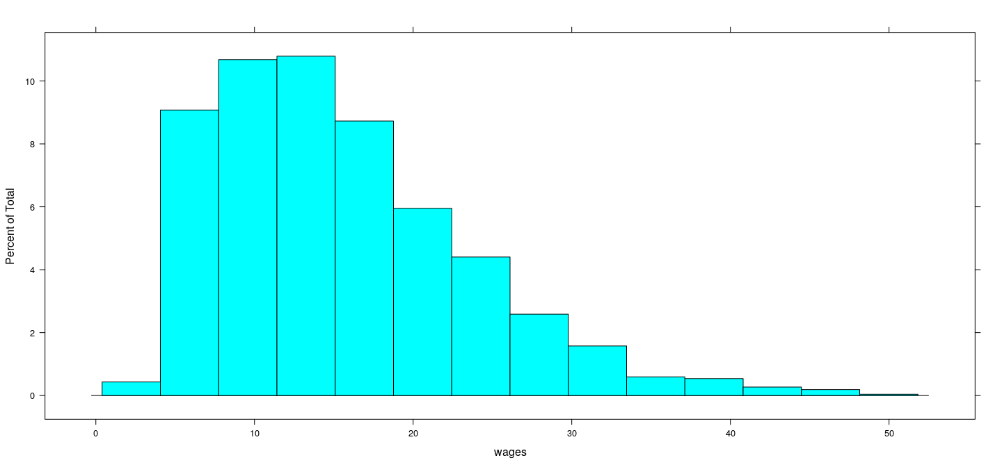
Distribution of wages (overall)
![plot of chunk unnamed-chunk-3]()
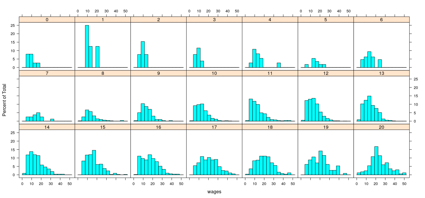
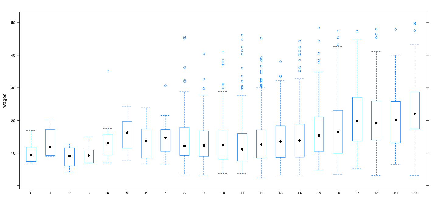
Distribution of wages (conditional on education)
![plot of chunk unnamed-chunk-4]()
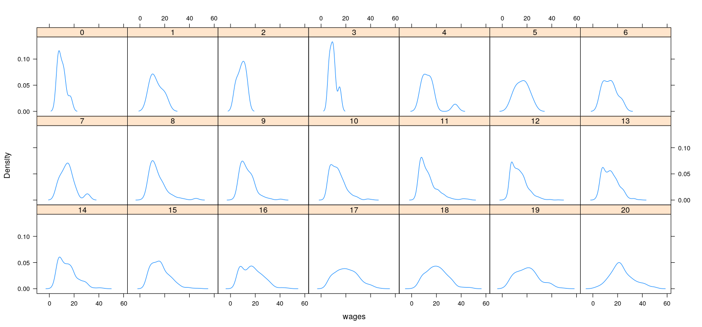
Distribution of wages (conditional on education)
![plot of chunk unnamed-chunk-5]()
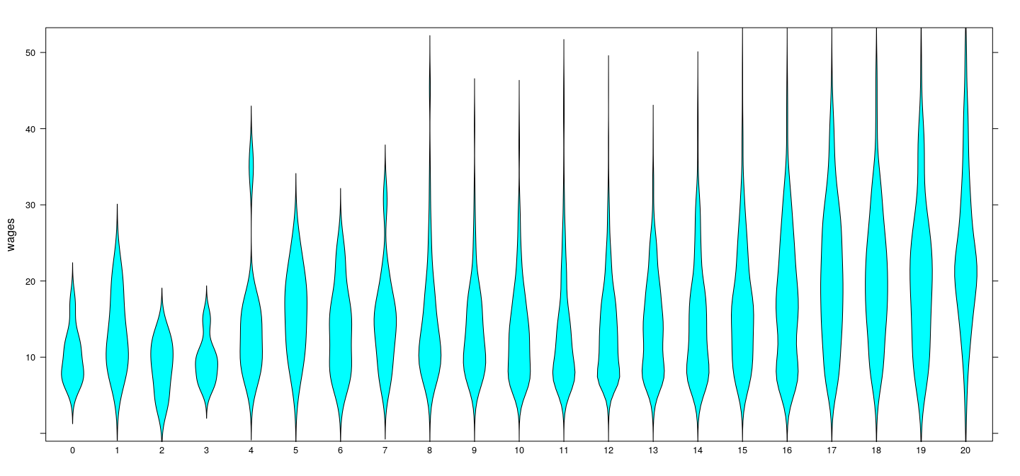
Distribution of wages (conditional on education)
![plot of chunk unnamed-chunk-6]()
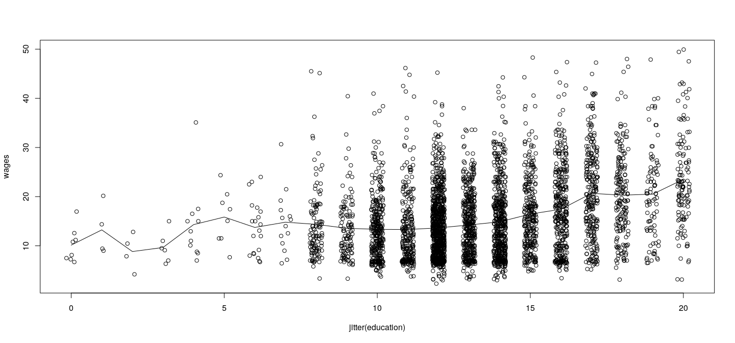
More direct comparison
![plot of chunk unnamed-chunk-7]()
More direct comparison
![plot of chunk unnamed-chunk-8]()
Pure error model
- Corresponding linear model is called the pure error model (assuming equal variance)
Call:
lm(formula = wages ~ education, data = SLID)

Residuals:
    Min      1Q  Median      3Q     Max
-17.649  -5.796  -1.005   4.133  34.139

Coefficients:
            Estimate Std. Error t value Pr(>|t|)
(Intercept)   5.0829     0.5304   9.584   <2e-16 ***
education     0.7848     0.0388  20.226   <2e-16 ***
---
Signif. codes:  0 '***' 0.001 '**' 0.01 '*' 0.05 '.' 0.1 ' ' 1

Residual standard error: 7.5 on 4012 degrees of freedom
  (3411 observations deleted due to missingness)
Multiple R-squared:  0.09253,   Adjusted R-squared:  0.09231
F-statistic: 409.1 on 1 and 4012 DF,  p-value: < 2.2e-16
Pure error model
Call:
lm(formula = wages ~ factor(education), data = SLID)

Residuals:
    Min      1Q  Median      3Q     Max
-20.393  -5.670  -1.067   4.060  32.834

Coefficients:
                    Estimate Std. Error t value Pr(>|t|)
(Intercept)          10.1375     2.6133   3.879 0.000107 ***
factor(education)1    3.1000     4.5264   0.685 0.493470
factor(education)2   -1.3025     4.5264  -0.288 0.773551
factor(education)3   -0.4808     3.9920  -0.120 0.904132
factor(education)4    4.1743     3.4346   1.215 0.224297
factor(education)5    5.7100     3.6958   1.545 0.122429
factor(education)6    3.5995     3.0922   1.164 0.244463
factor(education)7    4.6654     3.2760   1.424 0.154496
factor(education)8    4.2245     2.7043   1.562 0.118327
factor(education)9    3.4266     2.7059   1.266 0.205455
factor(education)10   3.2118     2.6446   1.214 0.224633
factor(education)11   3.1782     2.6529   1.198 0.230994
factor(education)12   3.5089     2.6248   1.337 0.181355
factor(education)13   4.0991     2.6375   1.554 0.120223
factor(education)14   4.7441     2.6335   1.801 0.071714 .
factor(education)15   6.3196     2.6499   2.385 0.017133 *
factor(education)16   7.3000     2.6438   2.761 0.005786 **
factor(education)17  10.5326     2.6545   3.968 7.38e-05 ***
factor(education)18  10.1605     2.6714   3.803 0.000145 ***
factor(education)19  10.3711     2.7322   3.796 0.000149 ***
factor(education)20  13.3853     2.6970   4.963 7.23e-07 ***
---
Signif. codes:  0 '***' 0.001 '**' 0.01 '*' 0.05 '.' 0.1 ' ' 1

Residual standard error: 7.392 on 3993 degrees of freedom
  (3411 observations deleted due to missingness)
Multiple R-squared:  0.1227,    Adjusted R-squared:  0.1183
F-statistic: 27.93 on 20 and 3993 DF,  p-value: < 2.2e-16
Pure error model
Analysis of Variance Table

Response: wages
                    Df Sum Sq Mean Sq F value    Pr(>F)
factor(education)   20  30522 1526.08  27.931 < 2.2e-16 ***
Residuals         3993 218164   54.64
---
Signif. codes:  0 '***' 0.001 '**' 0.01 '*' 0.05 '.' 0.1 ' ' 1
Analysis of Variance Table

Model 1: wages ~ education
Model 2: wages ~ factor(education)
  Res.Df    RSS Df Sum of Sq      F    Pr(>F)
1   4012 225674
2   3993 218164 19    7510.3 7.2347 < 2.2e-16 ***
---
Signif. codes:  0 '***' 0.001 '**' 0.01 '*' 0.05 '.' 0.1 ' ' 1
Pure error model
![plot of chunk unnamed-chunk-12]()
Pure error model
Such comparison possible when lots of data, few unique covariate values
Can be used to assess “non-linearity”
But need graphical tools to assess
- Skewness
- Multiple modes
- “Heavy” tails
- Unequal variance / spread
But what can we do when covariate \(x\) is continuous?
weight ~ heightprestige ~ income
Continuous predictor
Even with large datasets, replicated \(x\) will be rare
We can still divide range of \(x\) into several bins
- Width of bin represents trade-off (for non-linear relationship)
- How “locally” we can estimate (bias of estimator)
- Number of data points (variance of estimator)
Example: Prestige data
![plot of chunk unnamed-chunk-13]()
Example: Prestige data
![plot of chunk unnamed-chunk-14]()
Example: Davis data
![plot of chunk unnamed-chunk-15]()
Example: Davis data
![plot of chunk unnamed-chunk-16]()
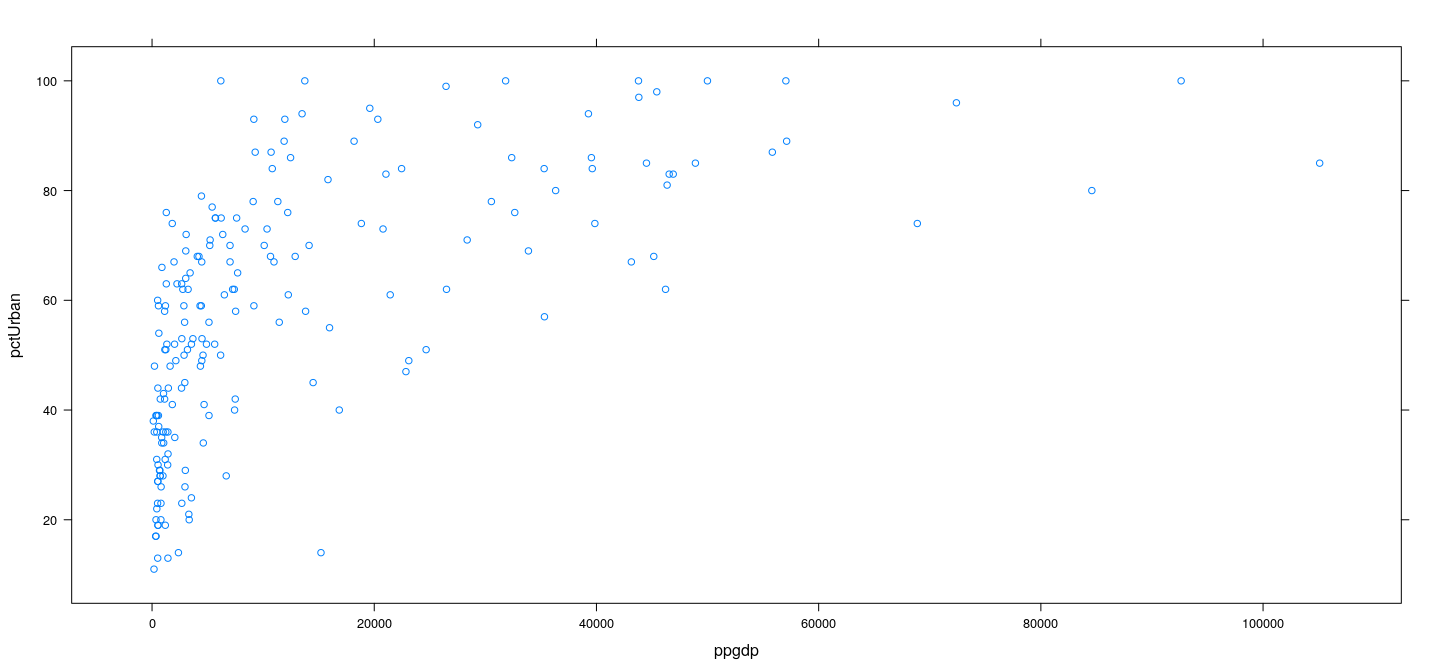
Example: UN data
![plot of chunk unnamed-chunk-17]()
Example: UN data
![plot of chunk unnamed-chunk-18]()
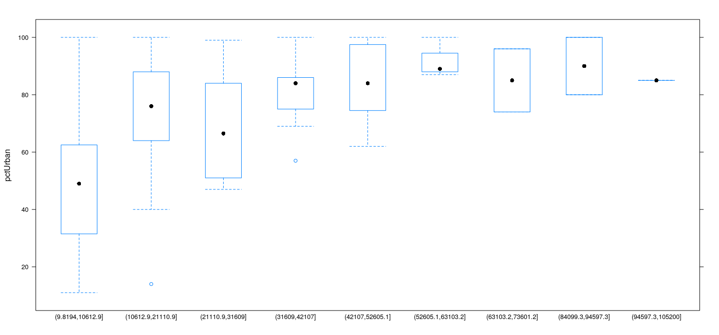
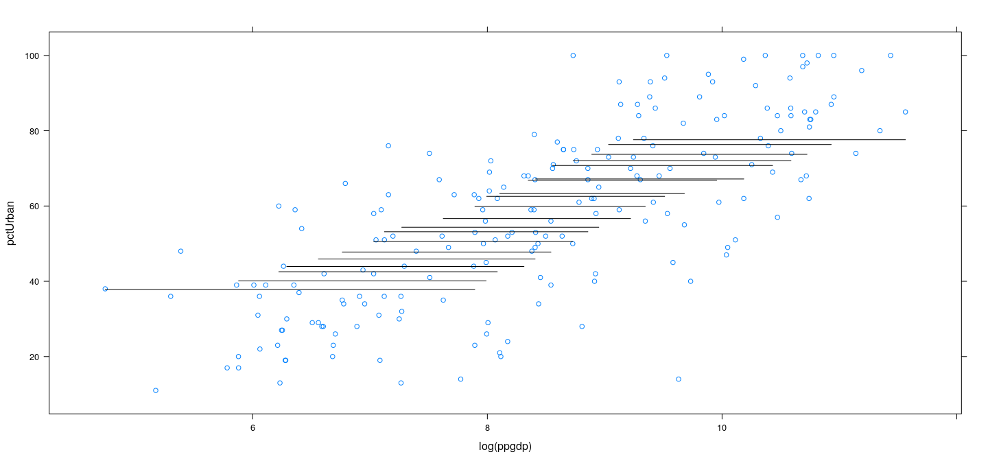
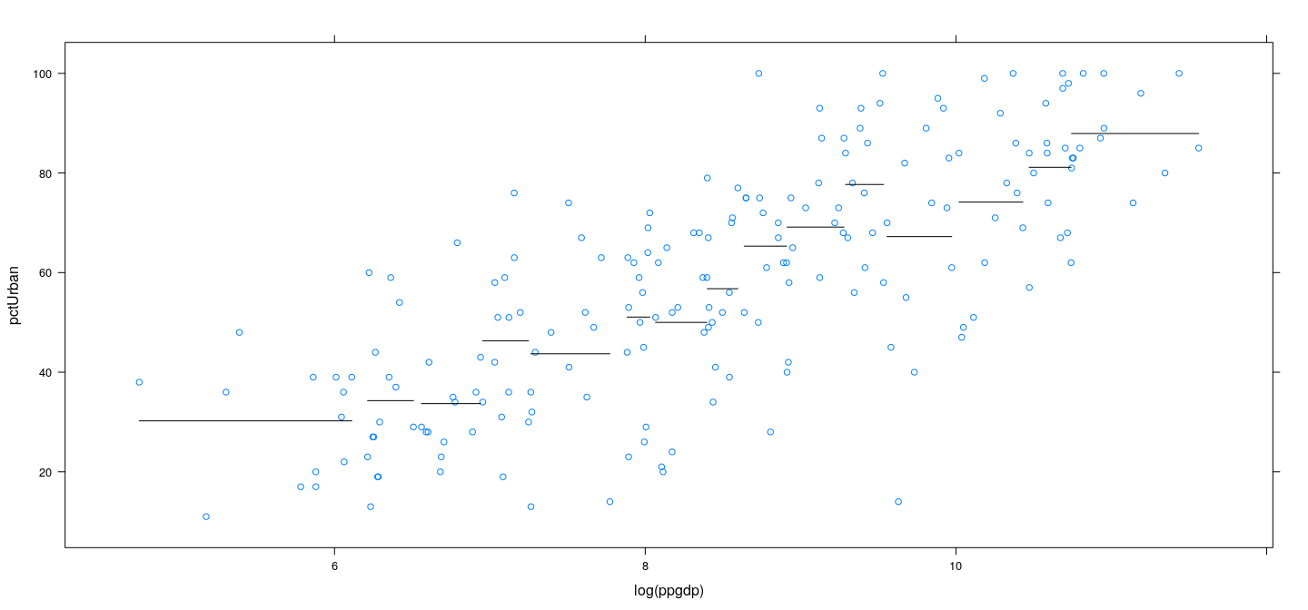
Choice of bin width - constant vs variable
Example: UN data — box and whisker plots
![plot of chunk unnamed-chunk-20]()
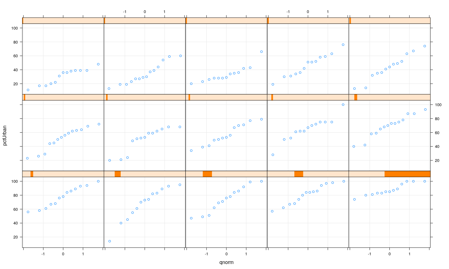
Example: UN data — Q-Q plots
![plot of chunk unnamed-chunk-21]()
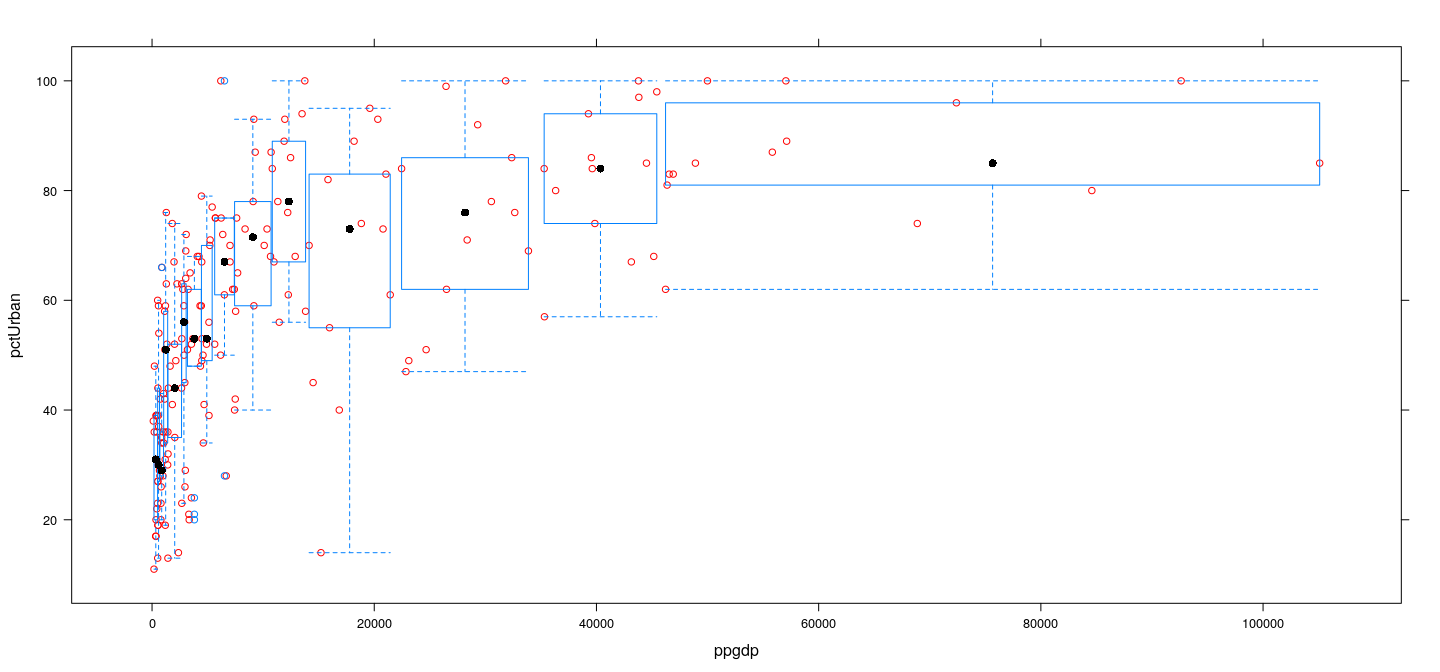
Assessing linearity
![plot of chunk unnamed-chunk-23]()
- Can summarize distribution in each bin my mean or median (and possibly standard deviation to assess non-constant variance)
Estimating conditional mean: a local binning approach
Model: \(Y_i = f(x_i) + \varepsilon_i\)
Interested in estimating \(f(x) = E(Y|x)\) for various \(x\)
Approach: Estimate \(f(x)\) locally by fitting mean or linear regression within bin
- Window size represents trade-off
- Larger window means more data points
- More data points means lower variance
- But larger window means larger bias
- Specifically, estimate is biased if \(f\) is non-linear, or if \(x\) is not uniformly distributed
Bias-variance trade-off — large data
Any reasonable method should at least be consistent
In other words, if we want to estimate \(E(Y|x)\), we should have \[
\hat{E}_n(Y|x) \to E(Y|x) \text{ as } n \to \infty
\]
Bias-variance trade-off — large data
If \(f(x) = E(Y | x)\) is “smooth”, then for \(x_i\) in the same bin as \(x_0\),
\[
f(x_i) = f(x_0) + f'(x_0) (x_i - x_0) + h(x_i) (x_i - x_0)
\]
where \(h(\cdot)\) is such that \(\lim_{x\to x_0} h(x) = 0\) (Taylor’s Theorem)
\(Y_i = f(x_i) + \varepsilon_i\), so for \(x_i\) in the same bin as \(x_0\), \[
Y_i = f(x_0) + f'(x_0) (x_i - x_0) + h(x_i) (x_i - x_0) + \varepsilon_i
\]
and so
\[
\bar{Y} (x_0) = f(x_0) + f'(x_0) (\bar{x} - x_0) + \bar{\varepsilon} + \frac{1}{n} \sum_i h(x_i) (x_i - x_0)
\]
As \(n \to \infty\), \(x_i, \bar{x} \to x_0\), so \(\bar{Y} (x_0) \to f(x_0)\)
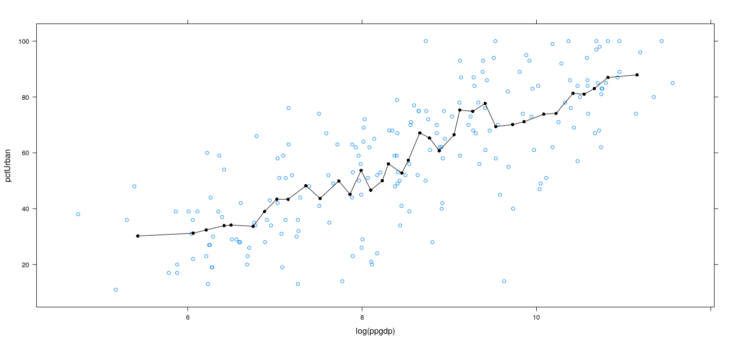
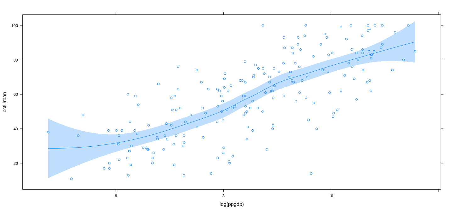
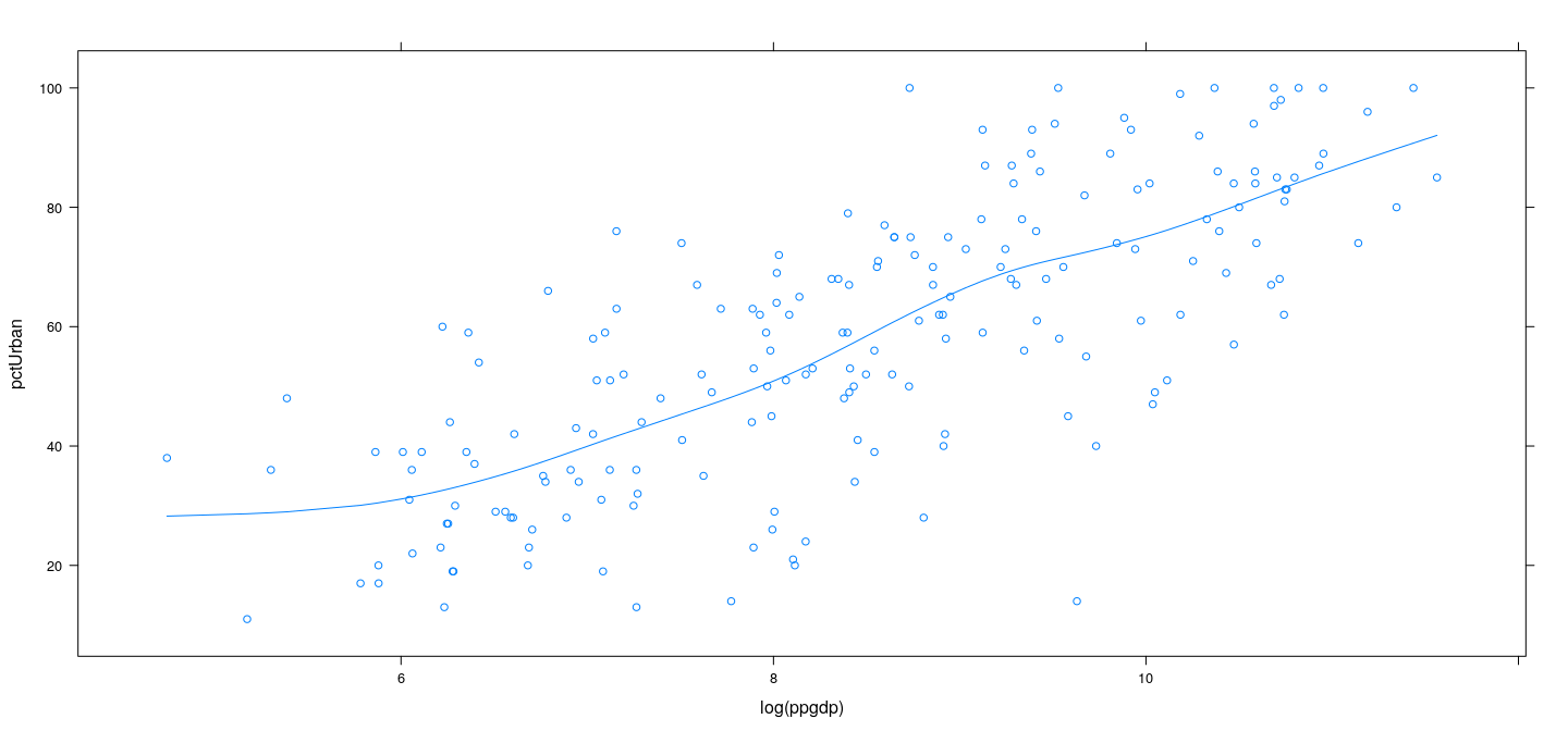
Example: UN data
![plot of chunk unnamed-chunk-24]()
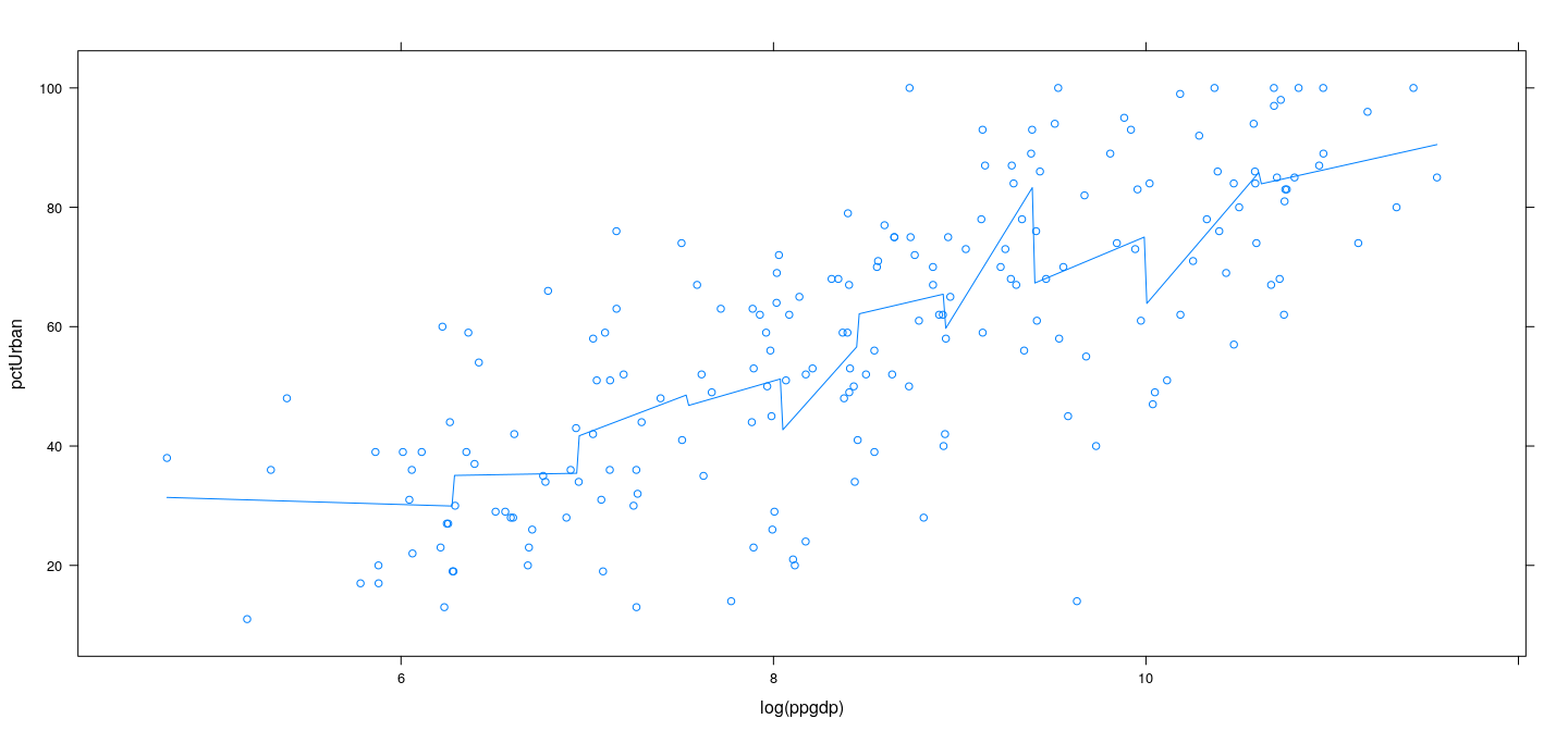
Example: UN data – overlapping bins
![plot of chunk unnamed-chunk-25]()
Example: UN data – overlapping bins
![plot of chunk unnamed-chunk-26]()
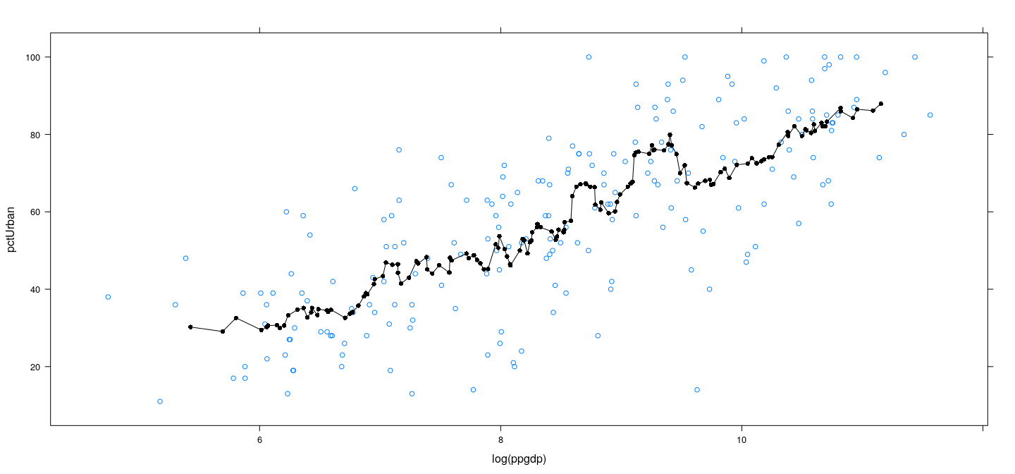
Example: UN data – more bins
![plot of chunk unnamed-chunk-27]()
Example: UN data – wider bins
![plot of chunk unnamed-chunk-28]()
Example: UN data – wider bins
![plot of chunk unnamed-chunk-29]()
Locally linear regression
Instead of \(\bar{Y}\), we could fit a linear regression model in each bin
\[
\hat{Y} (x_0) = \hat\alpha
\]
where \(\hat\alpha\) and \(\hat\beta\) are estimated by fitting the linear regression model (for all \(x_i\) in the same bin as \(x_0\))
\[
Y_i = \alpha + \beta (x_i - x_0) + \varepsilon_i
\]
- In general, the model could be a \(d\)-th “degree” polynomial
- \(d = 0\) : local mean
- \(d = 1\) : locally linear fit
- \(d = 2\) : locally quadratic fit
- Tuning parameter “span” : proportion of full data in each bin
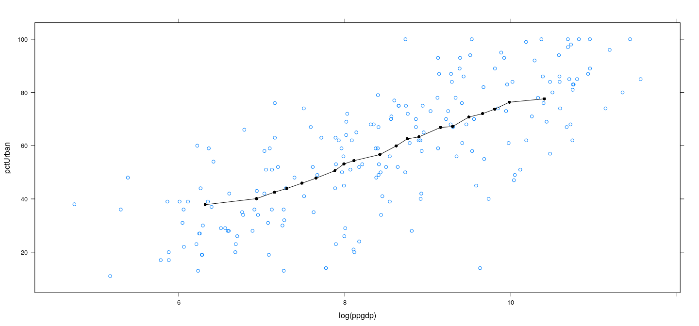
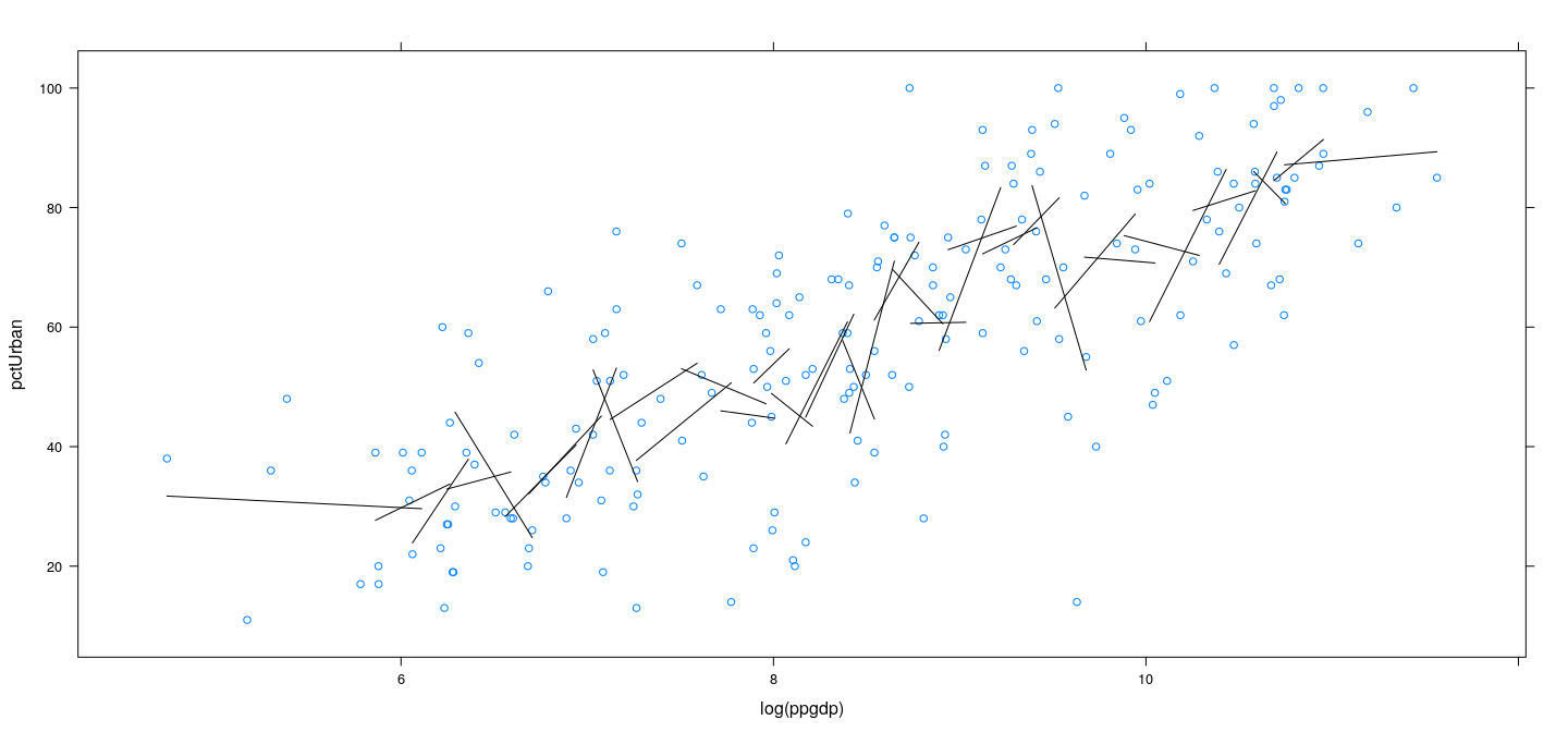
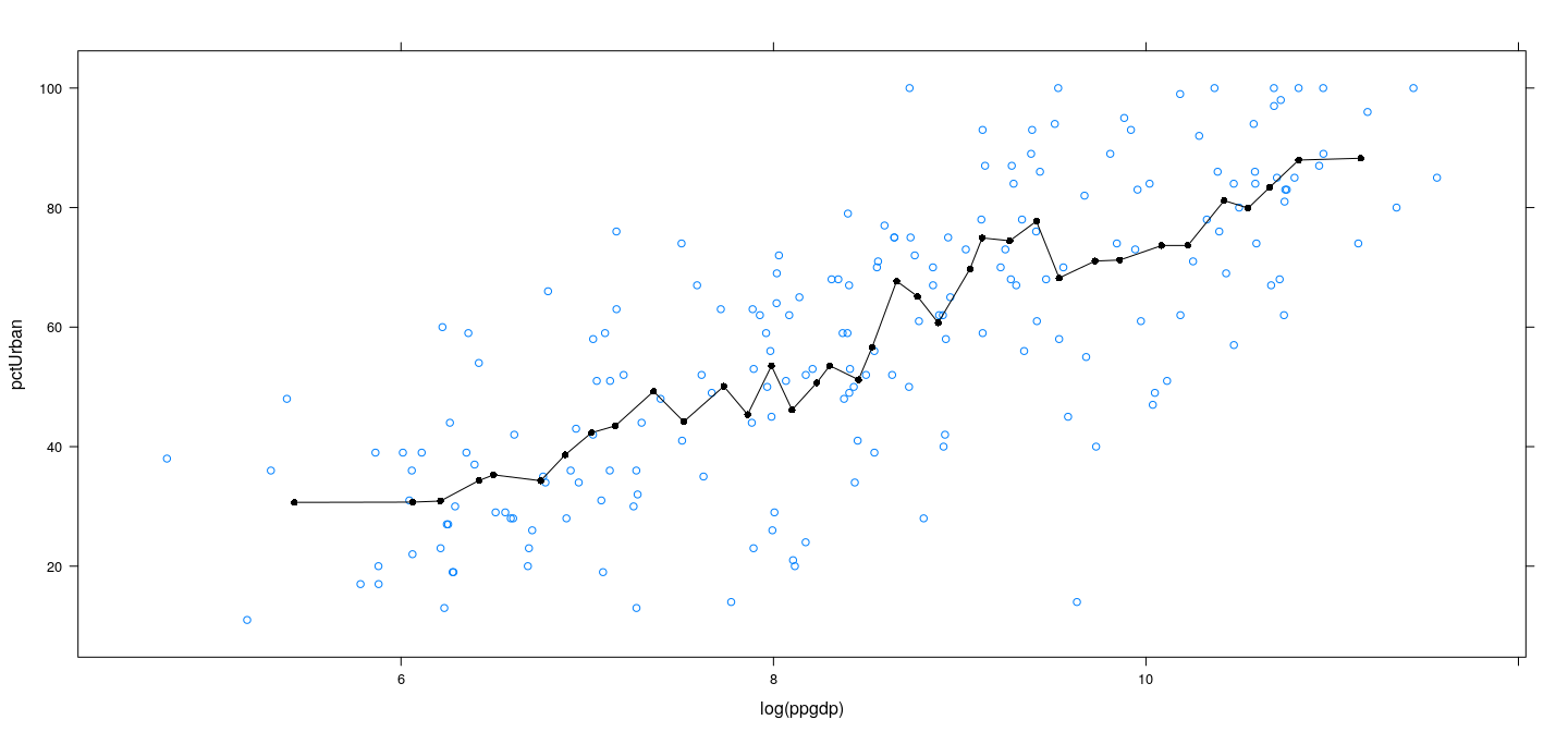
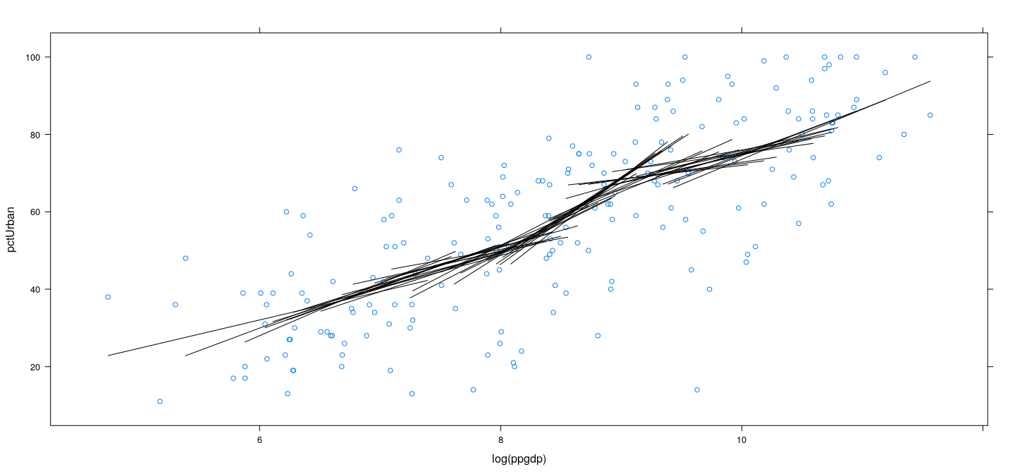
Example: UN data – locally linear
![plot of chunk unnamed-chunk-30]()
Example: UN data – locally linear
![plot of chunk unnamed-chunk-31]()
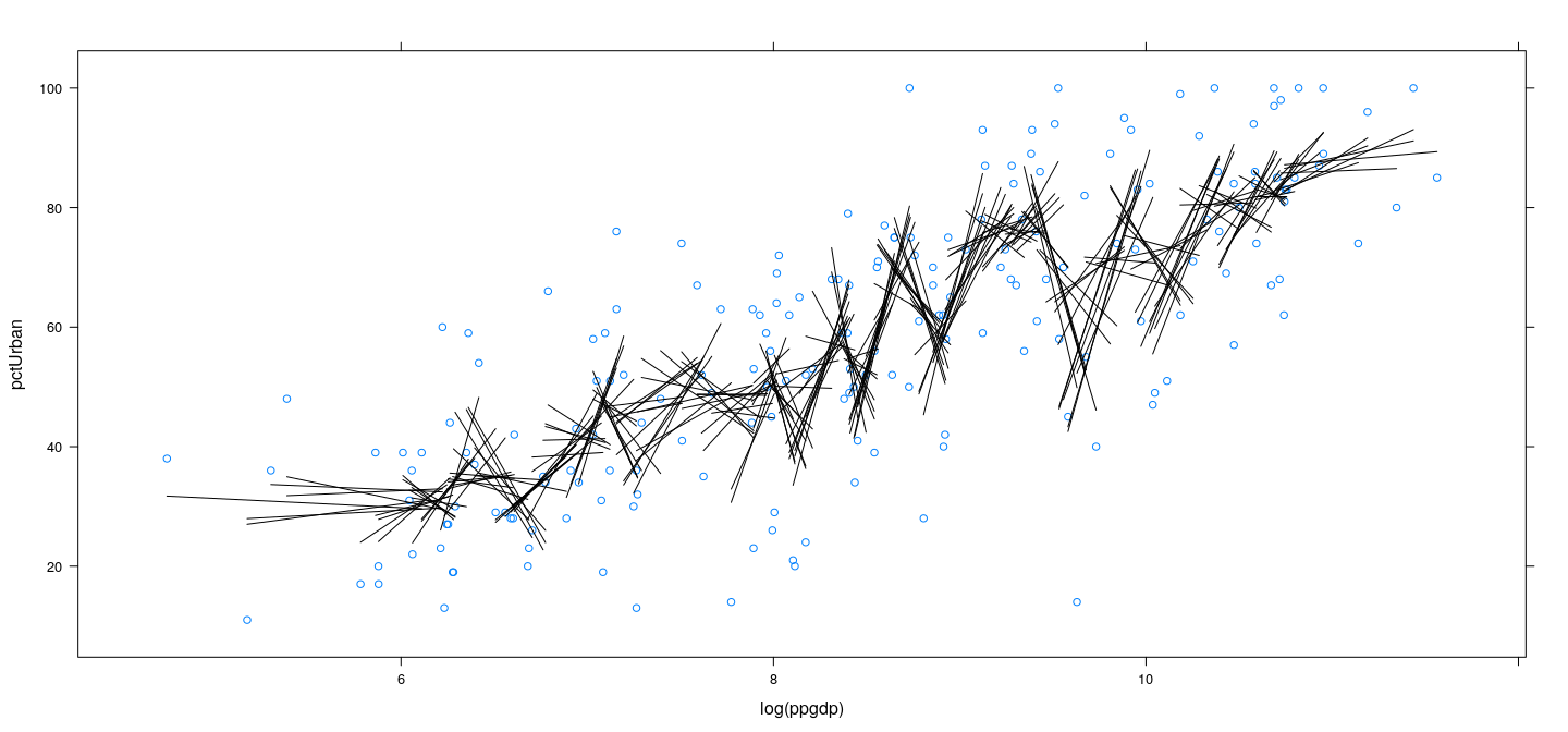
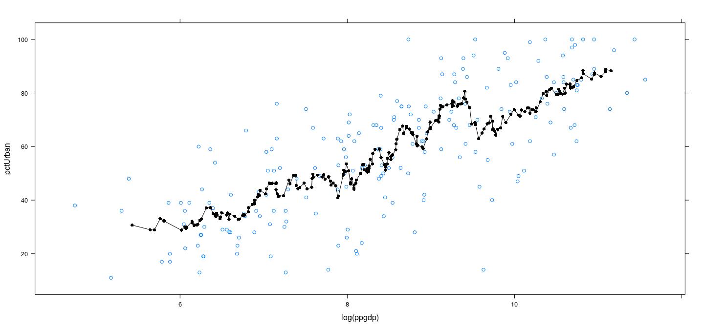
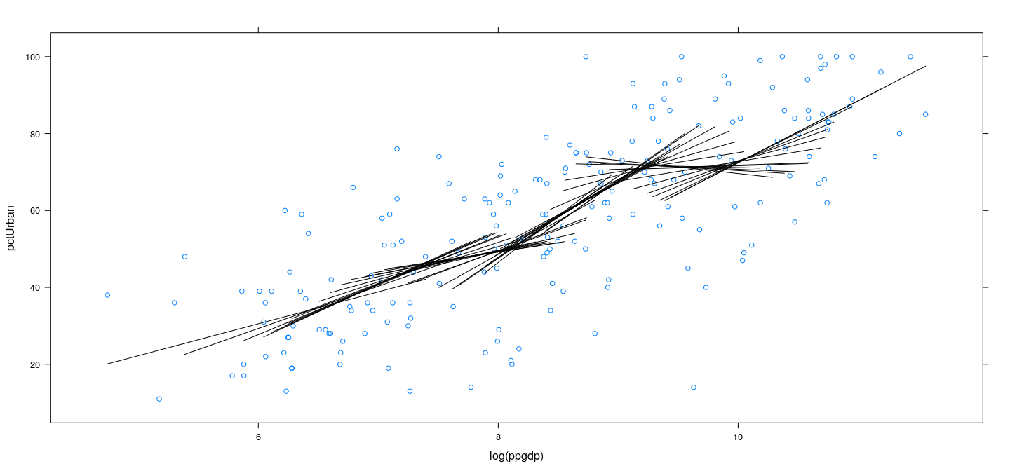
Example: UN data – locally linear with more bins
![plot of chunk unnamed-chunk-32]()
Example: UN data – locally linear with more bins
![plot of chunk unnamed-chunk-33]()
Example: UN data – locally linear with wider bins
![plot of chunk unnamed-chunk-34]()
Example: UN data – locally linear with wider bins
![plot of chunk unnamed-chunk-35]()
Adding weights
- Larger span gives
- Wider bins
- Smoother estimate of \(f(x) = E(Y|x)\)
- But more data points per bin (less “local”)
- One solution is to add weights (give more weightage to \(x_i\) near \(x_0\))
Weighted mean: \(\hat{Y} = \frac{\sum w_i Y_i}{ \sum w_i }\)
Weighted regression: Normal equations are given by \[
\mathbf{X}^T \mathbf{W} \mathbf{X} \widehat{\beta} = \mathbf{X}^T \mathbf{W} \mathbf{y}
\] where \(\mathbf{W}^{-1}\) is a diagonal matrix of inverse weights \(1/w_i^2\) (higher weight means less uncertainty).
- For example, \[
w_i = k((x_i - x_0) / h),
\] where
- \(2h\) is the bin width
- \(k(\cdot)\) is a symmetric weight function that is highest at \(0\) and decreases (usually to \(0\) at \(\pm h\))
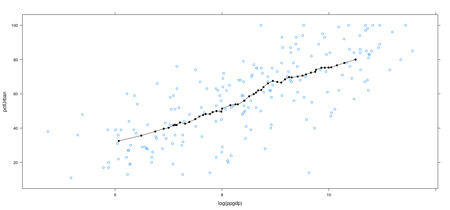
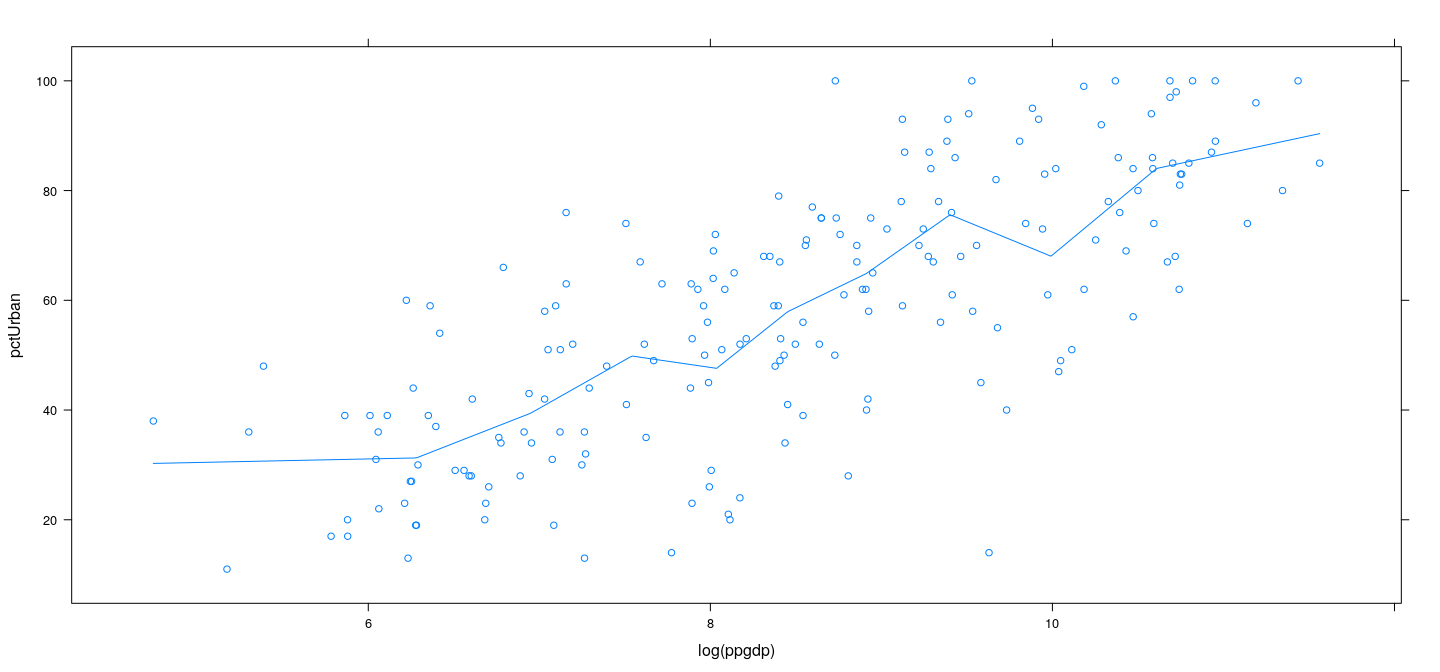
Example: UN data – locally weighted linear regression
![plot of chunk unnamed-chunk-36]()
Example: UN data – locally weighted linear regression
![plot of chunk unnamed-chunk-37]()
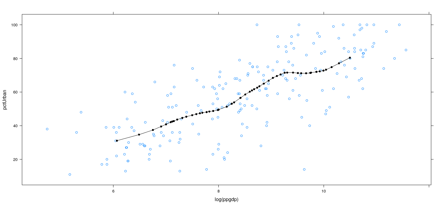
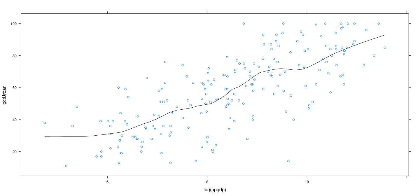
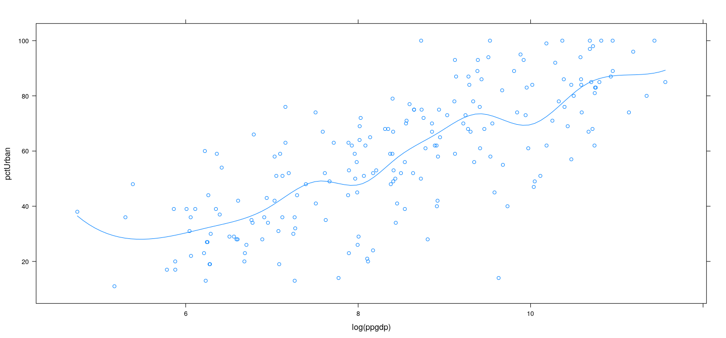
Example: UN data – LOWESS
![plot of chunk unnamed-chunk-38]()
LOWESS
Stands for “LOcally WEighted Scatterplot Smoother”
Can be viewed as \(k\) nearest neighbour weighted local polynomial regression
Main control parameters are span and degree
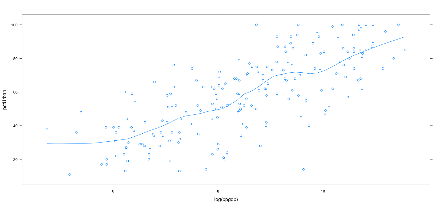
Example: UN data – LOWESS
![plot of chunk unnamed-chunk-40]()
Example: UN data – LOWESS
![plot of chunk unnamed-chunk-41]()
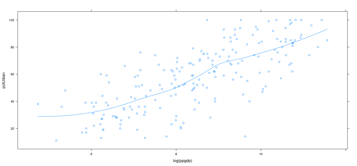
Example: UN data – LOWESS
![plot of chunk unnamed-chunk-42]()
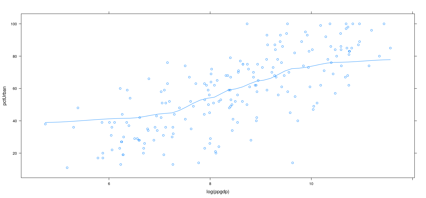
Example: UN data – LOWESS with local mean
![plot of chunk unnamed-chunk-43]()
Example: UN data – LOWESS with confidence band
![plot of chunk unnamed-chunk-44]()
Example: Davis data – LOWESS with least squares
![plot of chunk unnamed-chunk-45]()
Example: Davis data – LOWESS with robust regression
![plot of chunk unnamed-chunk-46]()
Example: Davis data – effect of span
![plot of chunk unnamed-chunk-47]()
Choice of span in LOWESS
The span (proportion of data in each bin) is an important tuning parameter
How do we choose span?
Generally speaking, cross-validation is often a useful strategy for choosing tuning parameters
Choose span to minimize \[
\sum_{i=1}^n (Y_i - \hat{Y}_{i(-i)})^2
\]
This is equivalent to maximixing predictive \(R^2\)
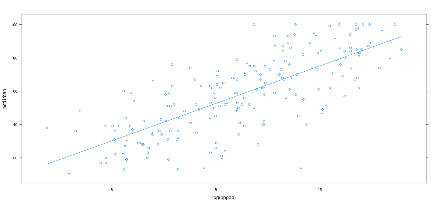
Parametric “smooth” regression
![plot of chunk unnamed-chunk-48]()
Parametric “smooth” regression
This can be viewed as a piecewise constant \(f(x)\)
Choose breakpoints (“knots”) \(-\infty = t_0 < t_1 < t_2 < \cdots < t_k = +\infty\)
Define \(Z_{ji} = 1\{ X_i \in (t_{j-1}, t_{j} ] \}\) for \(j = 1, 2, \dotsc, k\)
- Fit linear model \(\mathbf{y} = \mathbf{Z \beta} + \mathbf{\varepsilon}\) — this will give piecewise constant \(\hat{f}\)
Pieceise constant regression
pconst <- function(x, knots)
{
    Z <- matrix(0, length(x), length(knots) - 1)
    for (j in seq_len(length(knots)-1))
        Z[, j] <- ifelse(knots[j] < x & x <= knots[j+1], 1, 0)
    Z
}
lgdp.knots <- c(-Inf,
                quantile(log(UN$ppgdp), probs = seq(0.1, 0.9, by = 0.1), na.rm = TRUE),
                Inf)
Pieceise constant regression
![plot of chunk unnamed-chunk-51]()
Piecewise linear regression
Knots \(-\infty = t_0 < t_1 < t_2 < \cdots < t_k = +\infty\)
\(f(x) = \alpha_j + \beta_j x\) for \(x \in (t_{j-1}, t_{j} ]\) for \(j = 1, 2, \dotsc, k\)
Define \(Z_{ji} = 1\{ X_i \in (t_{j-1}, t_{j} ] \}\) for \(j = 1, 2, \dotsc, k\)
Additionally, define \(\tilde{Z}_{ji} = Z_{ji} x_i\) for \(j = 1, 2, \dotsc, k\)
Piecewise linear regression
![plot of chunk unnamed-chunk-53]()
Piecewise linear interpolating regression
This is the best (least squares) piecewise linear \(f(x)\) of the form \[
f(x) = \alpha_j + \beta_j x
\] for \(x \in (t_{j-1}, t_{j} ]\,,\, j = 1, 2, \dotsc, k\).
But we would prefer \(f\) to be continuous
Requires \(\alpha_j + \beta_j t_j = \alpha_{j+1} + \beta_{j+1} t_j\) for \(j = 1, 2, \dotsc, k-1\)
Equivalent formulation
\[
f(x) = \delta_0 + \gamma_0 x + \sum_{j=1}^{k-1} \gamma_j (x-t_j)_{+}
\]
where \(x_{+} = \max\{ 0, x \}\)
Piecewise linear regression
![plot of chunk unnamed-chunk-55]()
Natural generalization: piecewise quadratic interpolation
(with matching first derivatives)
\[
f(x) = \alpha_0 + \alpha_1 x + \beta_0 x^2 + \sum_{j=1}^{k-1} \beta_j (x-t_j)^2_{+}
\]
where \(x_{+} = \max\{ 0, x \}\)
Natural generalization: piecewise quadratic interpolation
![plot of chunk unnamed-chunk-57]()
Further generalization: piecewise cubic interpolation
(with matching second derivatives)
\[
f(x) = \alpha_0 + \alpha_1 x + \alpha_2 x^2 + \beta_0 x^3 + \sum_{j=1}^{k-1} \beta_j (x-t_j)^3_{+}
\]
where \(x_{+} = \max\{ 0, x \}\)
Further generalization: piecewise cubic interpolation
![plot of chunk unnamed-chunk-59]()
Also known as cubic spline regression
![plot of chunk unnamed-chunk-60]()
Regression with basis functions: background
Goal: Estimate best (least squares) \(\hat{f}\) within some class of functions
Example: “Interpolating splines” — piecewise cubic polynomials with continuous second derivatives
All the examples we have seen are vector spaces (for a fixed set of knots)
To find \(\hat{f}\) using a linear model, we need to find a basis
One example (for cubic interpolating splines) is \[
\{ 1, x, x^2, x^3 \} \cup \{ (x - t_j)^3_{+} : j = 1, ..., k-1 \}
\]
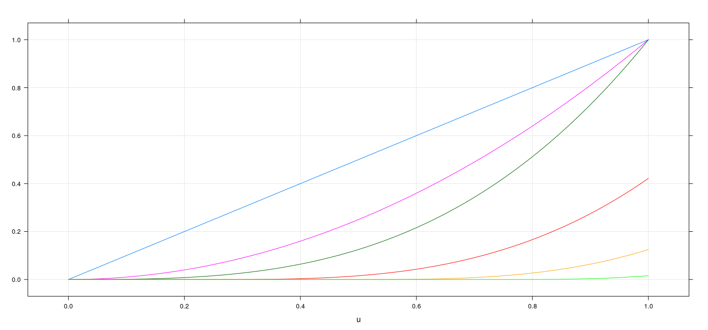
Plot of cubic spline basis functions
u <- seq(0, 1, length = 101)
m <- as.data.frame(pcubint(u, knots = c(-Inf, c(0.25, 0.5, 0.75, Inf))))
names(m) <- paste0("f", seq_len(ncol(m)))
xyplot(f1 + f2 + f3 + f4 + f5 + f6 ~ u, data = cbind(u, m), type = "l", ylab = NULL, grid = TRUE)
![plot of chunk unnamed-chunk-61]()
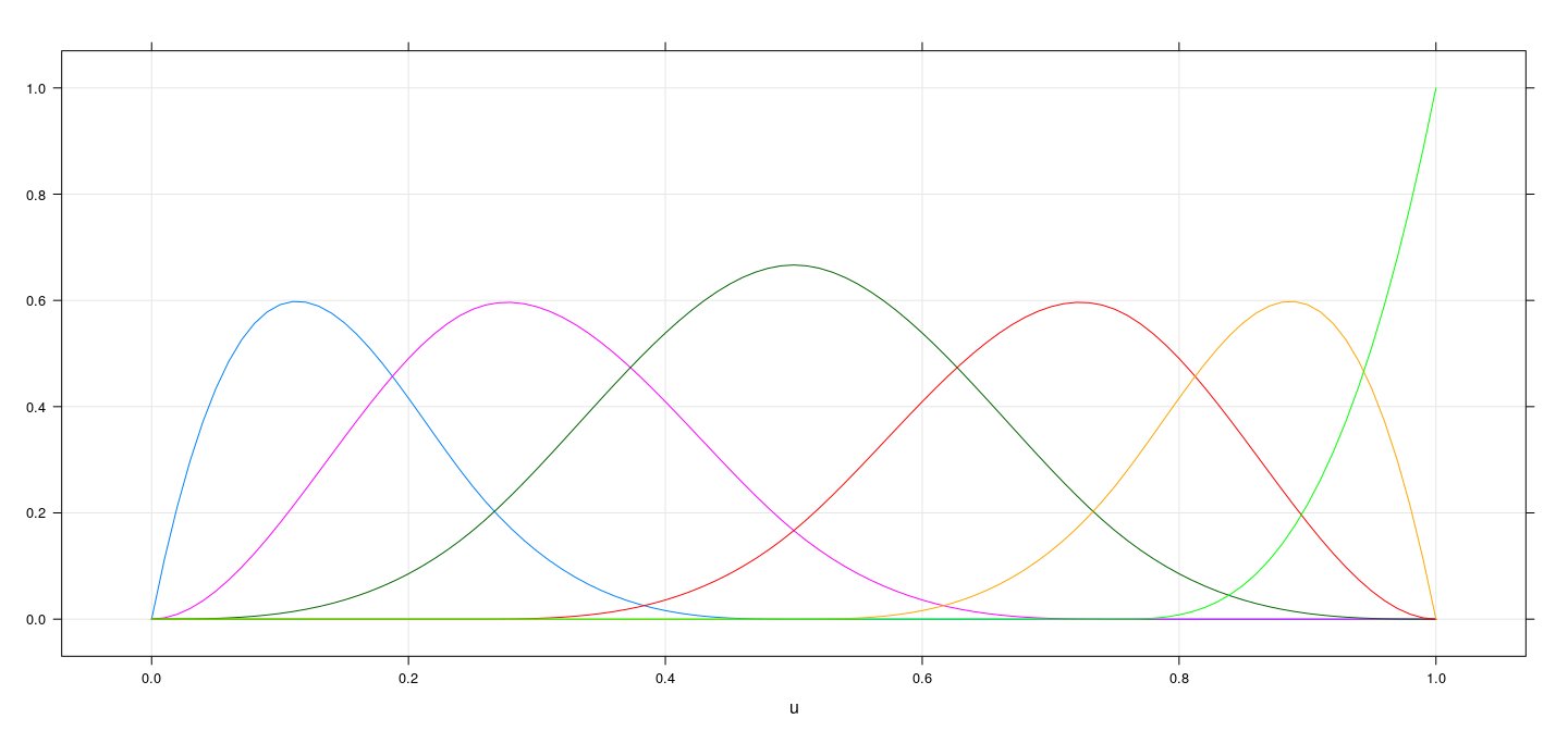
Alternative basis for cubic splines
u <- seq(0, 1, length = 101)
m <- as.data.frame(bs(u, knots = c(0.25, 0.5, 0.75)))
names(m) <- paste0("f", seq_len(ncol(m)))
xyplot(f1 + f2 + f3 + f4 + f5 + f6 ~ u, data = cbind(u, m), type = "l", ylab = NULL, grid = TRUE)
![plot of chunk unnamed-chunk-62]()
Basis splines in R
Available as the bs() function in package splines (degree 3, “cubic”, by default)
Usually specify df rather than explicit knots (tuning parameter providing flexibility)
Call:
lm(formula = pctUrban ~ 1 + bs(log(ppgdp), df = 6), data = UN)

Residuals:
    Min      1Q  Median      3Q     Max
-58.942  -9.267   0.426  11.094  38.561

Coefficients:
                        Estimate Std. Error t value Pr(>|t|)
(Intercept)               34.688     13.254   2.617 0.009573 **
bs(log(ppgdp), df = 6)1  -11.885     20.810  -0.571 0.568600
bs(log(ppgdp), df = 6)2    2.469     13.466   0.183 0.854691
bs(log(ppgdp), df = 6)3   21.769     14.884   1.463 0.145226
bs(log(ppgdp), df = 6)4   44.026     14.446   3.048 0.002631 **
bs(log(ppgdp), df = 6)5   46.601     16.149   2.886 0.004354 **
bs(log(ppgdp), df = 6)6   59.317     16.645   3.564 0.000462 ***
---
Signif. codes:  0 '***' 0.001 '**' 0.01 '*' 0.05 '.' 0.1 ' ' 1

Residual standard error: 15.65 on 192 degrees of freedom
  (14 observations deleted due to missingness)
Multiple R-squared:  0.5674,    Adjusted R-squared:  0.5539
F-statistic: 41.98 on 6 and 192 DF,  p-value: < 2.2e-16
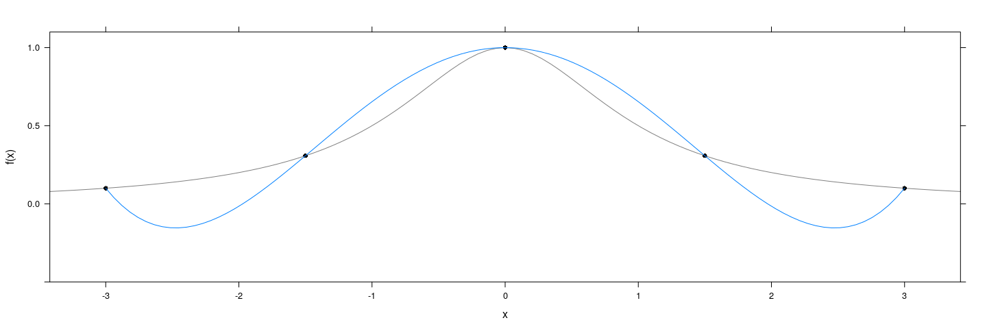
Why splines?
f <- function(x) 1 / (1 + x^2)
degree <- 4
x <- seq(-3, 3, length = degree + 1)
xyplot(f(x) ~ x, col = 1, pch = 16, ylim = c(-0.5, 1.1)) +
    layer_(panel.curve(f, type = "l", col = "grey50")) +
        layer(panel.smoother(x, y, method = "lm", form = y ~ poly(x, degree), se = FALSE))
![plot of chunk unnamed-chunk-64]()
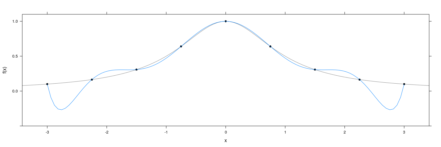
Why splines?
f <- function(x) 1 / (1 + x^2)
degree <- 8
x <- seq(-3, 3, length = degree + 1)
xyplot(f(x) ~ x, col = 1, pch = 16, ylim = c(-0.5, 1.1)) +
    layer_(panel.curve(f, type = "l", col = "grey50")) +
        layer(panel.smoother(x, y, method = "lm", form = y ~ poly(x, degree), se = FALSE))
![plot of chunk unnamed-chunk-65]()
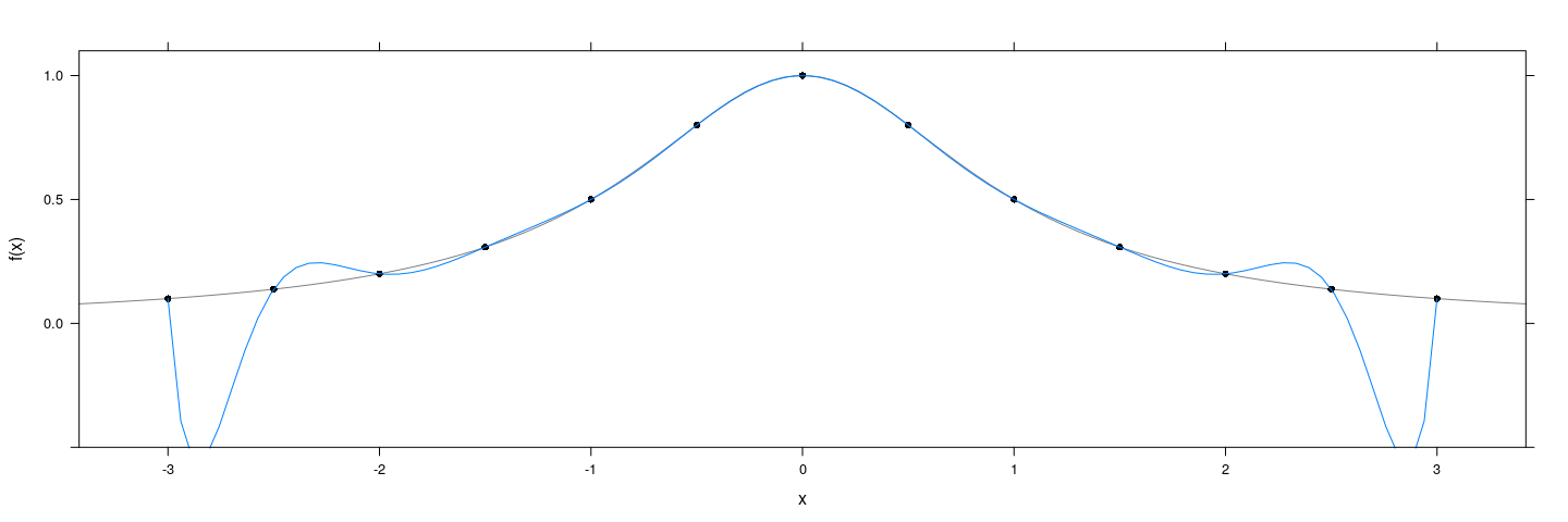
Why splines?
f <- function(x) 1 / (1 + x^2)
degree <- 12
x <- seq(-3, 3, length = degree + 1)
xyplot(f(x) ~ x, col = 1, pch = 16, ylim = c(-0.5, 1.1)) +
    layer_(panel.curve(f, type = "l", col = "grey50")) +
        layer(panel.smoother(x, y, method = "lm", form = y ~ poly(x, degree), se = FALSE))
![plot of chunk unnamed-chunk-66]()
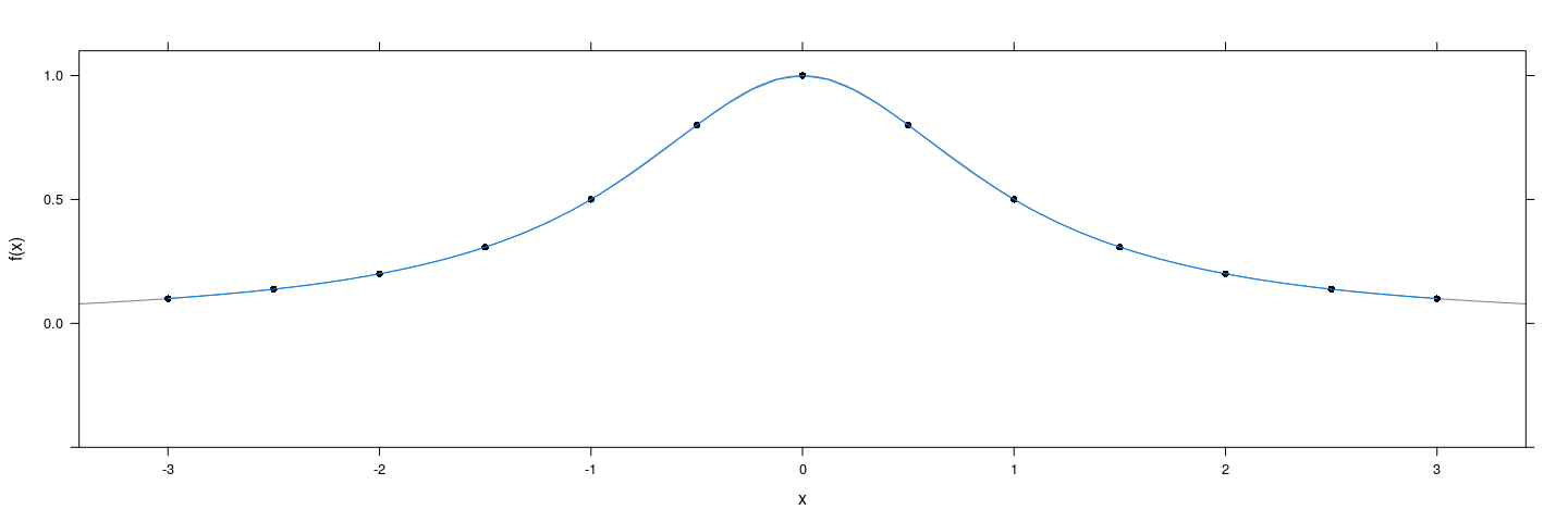
Why splines?
![plot of chunk unnamed-chunk-67]()
An interesting property of interpolating splines
Consider finding \(f: [a,b] \to \mathbb{R}\) interpolating the points \(\{ (x_i, y_i ) : x_i \in [a, b] \}\) that minimizes
\[
\int_{a}^{b} (f^{\prime\prime}(t))^2 dt \quad\quad \text{(roughness penalty)}
\]
in the class of functions with continuous second derivative
- The solution is a “natural” cubic spline
- “Natural” because the solution is linear outside the range of the knots
Smoothing splines
A non-parametric regression approach motivated by this:
Find \(f\) to minimize (given \(\lambda > 0\))
\[
\sum_i (y_i - f(x_i))^2 + \lambda \int_{a}^{b} (f^{\prime\prime}(t))^2 dt
\]
- The solution is a “natural” cubic spline
- \(\lambda\) represents a tuning parameter (smoothness vs flexibility)
- \(\lambda\) is usually chosen by a form of cross-validation
- The mathematical analysis of smoothing splines is relatively complicated (will not discuss)
Smoothing splines in R
Call:
smooth.spline(x = log(ppgdp), y = pctUrban, df = 6)

Smoothing Parameter  spar= 1.034826  lambda= 0.004116211 (12 iterations)
Equivalent Degrees of Freedom (Df): 6.000823
Penalized Criterion (RSS): 46566.24
GCV: 1031.185
Call:
smooth.spline(x = log(ppgdp), y = pctUrban)

Smoothing Parameter  spar= 1.499952  lambda= 9.443731 (25 iterations)
Equivalent Degrees of Freedom (Df): 2.030403
Penalized Criterion (RSS): 47818.1
GCV: 986.3203
Smoothing splines in R
![plot of chunk unnamed-chunk-69]()
Smoothing splines in R
![plot of chunk unnamed-chunk-70]()
Summary: smooth regression for non-linear expectation function
Focuses on estimating \(f(x) = E(Y | X=x)\)
Several methods available, both non-parametric and parametric
Usually involves tuning parameter that needs to be chosen
Can be used to visually diagnose non-linearity of \(f(x)\)
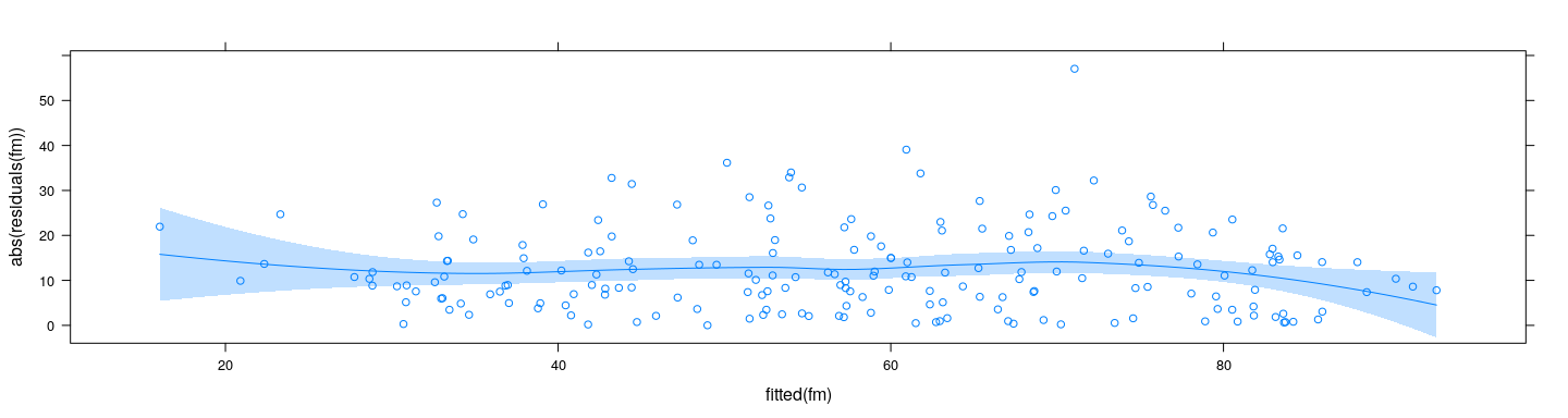
What about non-constant variance?
![plot of chunk unnamed-chunk-71]()
Summary: smooth regression for non-linear expectation function
Focuses on estimating \(f(x) = E(Y | X=x)\)
Several methods available, both non-parametric and parametric
Usually involves tuning parameter that needs to be chosen
Can be used to visually diagnose non-linearity of \(f(x)\)
Can also be used to diagnose heteroscedasticity