Robust Regression
Deepayan Sarkar
Motivation
Least squares regression is sensitive to violation of assumptions
Individual high-leverage points can substantially influence inference
Specifically, least squares is vulnerable when error distribution is heavy-tailed
- Another alternative is to consider procedures that systematically guard against outliers
Motivation: Location and scale
- A more familiar example before considering the regression problem:
\[
X_1, \dotsc, X_n \sim N(\mu, \sigma^2)
\]
[1] 4.2967261 0.8741864 7.7031483 -0.0853126 2.5003953 5.6141429 8.6149780 11.0482167 -1.9215526 -0.3005308
| Mean |
mean(x) |
3.8344398 |
| Median |
median(x) |
3.3985607 |
| Trimmed mean |
mean(x, trim = 0.25) |
3.4838811 |
Robust estimation of location
Relative efficiency
\[
RE(T_1; T_2) = \frac{V(T_2)}{V(T_1)}
\]
For biased estimators, variance could be replaced by MSE
\(T_2\) is usually taken to be the optimal estimator, if one is available
What are relative efficiencies of median and trimmed mean?
Instead of trying to obtain variances theoretically (which is often difficult), we could use simulation to get a rough idea
Relative efficiency
sampling.variance <- function(estimator, rfun, n, NREP = 10000)
{
    var(replicate(NREP, estimator(rfun(n))))
}
trim.mean <- function(x) mean(x, trim = 0.25)
rdist <- function(n) rnorm(n, mean = 5, sd = 3)
var.mean <- sampling.variance(mean, rdist, n = 10)
var.median <- sampling.variance(median, rdist, n = 10)
var.tmean <- sampling.variance(trim.mean, rdist, n = 10)
round(100 * var.mean / var.median)
[1] 74
[1] 91
Asymptotic relative efficiency
\(ARE(T_1; T_2)\) is the limiting value of relative efficiency as \(n \to \infty\)
[1] 63
[1] 84
For comparison, the exact \(ARE\) of the median is \(\frac{2}{\pi} = 63.6\%\)
This is when the data comes from a normal distribution
Relative efficiency for heavier tails
- Suppose errors are instead from \(t\) with 5 degrees of freedom
[1] 96
[1] 121
Winsorized trimmed mean
- Similar to trimmed mean, but replaces trimmed observations by nearest untrimmed observation
[1] 91
[1] 117
Relative efficiency for contamination
Another “departure” model: contamination
Suppose data is a mixture of \(N(\mu, \sigma^2)\) with probability \(1-\epsilon\) and \(N(\mu, 9\sigma^2)\) with probability \(\epsilon\)
rdist <- function(n) rnorm(n, mean = 5, sd = ifelse(runif(n) < 0.01, 3, 1)) # 1% contamination
var.mean <- sampling.variance(mean, rdist, n = 5000)
var.median <- sampling.variance(median, rdist, n = 5000)
var.tmean <- sampling.variance(trim.mean, rdist, n = 5000)
round(100 * var.mean / c(median = var.median, trim.mean = var.tmean))
   median trim.mean
       69        92
rdist <- function(n) rnorm(n, mean = 5, sd = ifelse(runif(n) < 0.05, 3, 1)) # 5% contamination
var.mean <- sampling.variance(mean, rdist, n = 5000)
var.median <- sampling.variance(median, rdist, n = 5000)
var.tmean <- sampling.variance(trim.mean, rdist, n = 5000)
round(100 * var.mean / c(median = var.median, trim.mean = var.tmean))
   median trim.mean
       82       108
Sensitivity / influence function
\[
SC(x; x_1, \dotsc, x_{n-1}, T) = \frac{ T(x_1, \dotsc, x_{n-1}, x) - T(x_1, \dotsc, x_{n-1}) }{ 1/n }
\]
We are usually interested in limiting behaviour as \(n \to \infty\)
The population version, independent of the sample \(x_1, \dotsc, x_{n-1}\), is known as the influence function
\[
IF(x; F, T) = \lim_{\epsilon \to 0} \frac{ T( (1-\epsilon) F + \epsilon \delta_x) - T(F) }{\epsilon}
\]
- Here \(\delta_x\) is a point mass at \(x\)
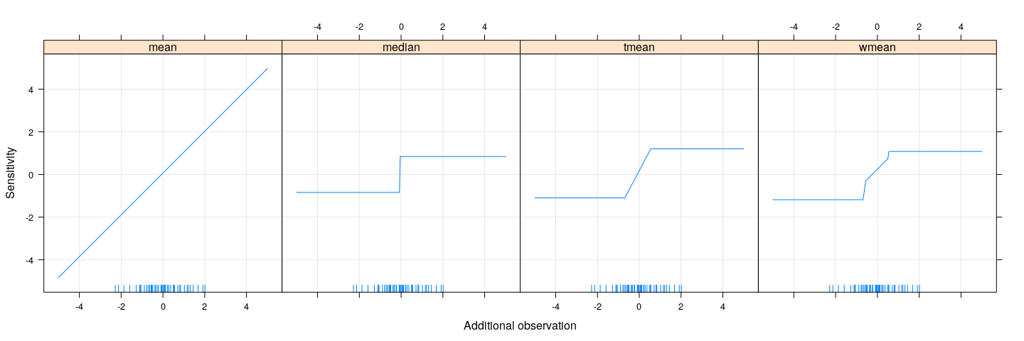
Sensitivity / influence function
    Min.  1st Qu.   Median     Mean  3rd Qu.     Max.
-2.28099 -0.61800 -0.06070 -0.06727  0.51522  2.01596
xx <- seq(-5, 5, 0.01)
sensitivity <-
    data.frame(xx = xx,
               mean = n * (sapply(xx, function(xnew) mean(c(x, xnew))) - mean(x)),
               median = n * (sapply(xx, function(xnew) median(c(x, xnew))) - median(x)),
               tmean = n * (sapply(xx, function(xnew) trim.mean(c(x, xnew))) - trim.mean(x)),
               wmean = n * (sapply(xx, function(xnew) win.mean(c(x, xnew))) - win.mean(x)))
Sensitivity / influence function
![plot of chunk unnamed-chunk-8]()
Breakdown point
Defined as the proportion of the sample size that must be perturbed to make the estimate unbounded
50% is the best we can hope for
For location, mean has 0% breakdown point (one out of \(n\)), median has 50%.
Relative efficiency for estimators of scale
rdist <- function(n) rnorm(n, mean = 5)                # Normal
var.T1 <- sampling.variance(T1, rdist, n = 5000)
var.T2 <- sampling.variance(T2, rdist, n = 5000)
var.T3 <- sampling.variance(T3, rdist, n = 5000)
var.T4 <- sampling.variance(T4, rdist, n = 5000)
round(100 * var.T1 / c(mean.abs.dev = var.T2, median.abs.dev = var.T3, iqr = var.T4))
  mean.abs.dev median.abs.dev            iqr
            89             38             38
rdist <- function(n) rnorm(n, mean = 5, sd = ifelse(runif(n) < 0.01, 3, 1)) # 1% Contamination
var.T1 <- sampling.variance(T1, rdist, n = 5000)
var.T2 <- sampling.variance(T2, rdist, n = 5000)
var.T3 <- sampling.variance(T3, rdist, n = 5000)
var.T4 <- sampling.variance(T4, rdist, n = 5000)
round(100 * var.T1 / c(mean.abs.dev = var.T2, median.abs.dev = var.T3, iqr = var.T4))
  mean.abs.dev median.abs.dev            iqr
           152             70             70
M-estimators
- Most common location estimators can be expressed as M-estimators (MLE-like)
\[
T(x_1, \dotsc, x_n) = \arg \min_{\theta} \sum_{i=1}^n \rho(x_i, \theta)
\]
For MLE, \(\rho(x_i, \theta)\) is the negative log-density, but \(\rho\) need not correspond to a likelihood
If \(\psi(x_i, \theta) = \frac{d}{d\theta} \rho(x_i, \theta)\) exists, then \(T\) is the solution to the score equation
\[
\sum_{i=1}^n \psi(x_i, \theta) = 0
\]
We usually consider loss functions of the form \(\rho(x - \theta)\)
Corresponding \(\psi\) function is \(\psi(x - \theta) = \rho^{\prime}(x - \theta)\) (disregarding change in sign)
This easily generalizes to vector parameters
M-estimators
\[
\rho(x - \theta) = (x-\theta)^2, \quad \psi(x - \theta) = 2 (x-\theta)
\]
- Median (ignoring non-differentiability of \(\lvert x \rvert\) at 0)
\[
\rho(x - \theta) = \lvert x-\theta \rvert, \quad \psi(x - \theta) = \text{sign}(x-\theta)
\]
- Trimmed mean (for some \(c\), ignoring dependence of \(c\) on the data)
\[
\rho(x - \theta) = \begin{cases}
(x-\theta)^2 & \lvert x - \theta \rvert \leq c \\
c^2 & \text{otherwise}
\end{cases}
\]
\[
\psi(x - \theta) = \begin{cases}
2 (x-\theta) & \lvert x - \theta \rvert \leq c \\
0 & \text{otherwise}
\end{cases}
\]
M-estimators
- Huber loss (similar to Winsorized trimmed mean)
\[
\rho(x - \theta) = \begin{cases}
(x-\theta)^2 & \lvert x - \theta \rvert \leq c \\
c (2 \lvert x-\theta \rvert - c) & \text{otherwise}
\end{cases}
\]
\[
\psi(x - \theta) = \begin{cases}
-2c & x - \theta < -c \\
2 (x-\theta) & \lvert x - \theta \rvert \leq c \\
2c & x - \theta > c
\end{cases}
\]
Can be thought of compromise between mean (squared error) and median (absolute error)
Estimator reduces to mean as \(c \to \infty\), median as \(c \to 0\)
\(\rho\) is differentiable everywhere
- Exercise: What do plots of \(\rho\) and \(\psi\) look like?
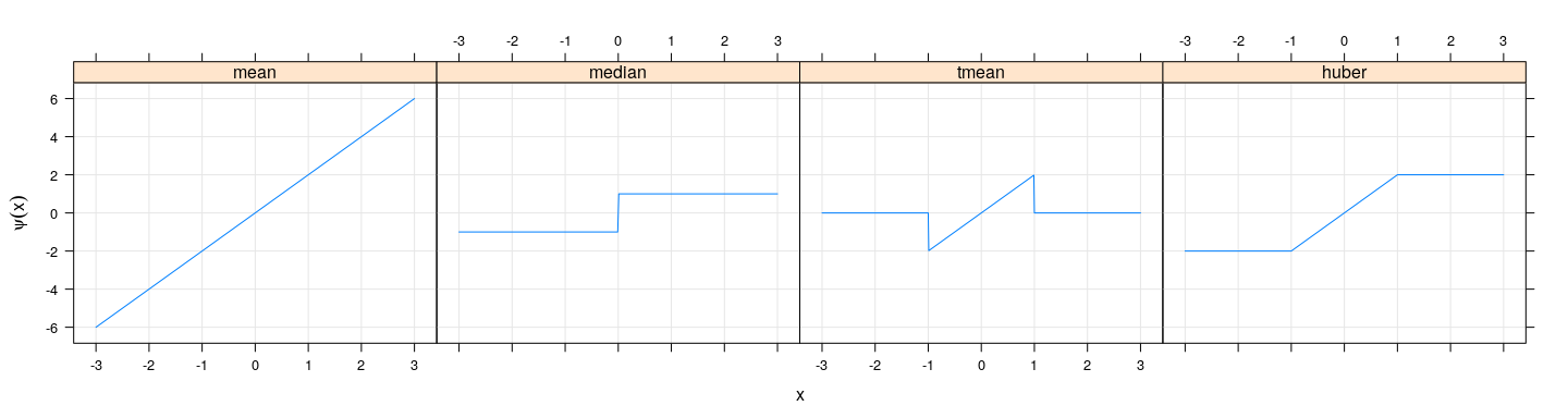
Influence function revisited
xx <- seq(-3, 3, 0.01)
sensitivity <-
    data.frame(xx = xx,
               mean = 2 * xx,
               median = sign(xx),
               tmean = ifelse(abs(xx) < 1, 2 * xx, 0),
               huber = ifelse(abs(xx) < 1, 2 * xx, 2 * sign(xx)))
xyplot(mean + median + tmean + huber ~ xx, sensitivity, type = "l", outer = TRUE,
       xlab = "x", ylab = expression(psi(x)), grid = TRUE)
![plot of chunk unnamed-chunk-12]()
- Turns out that the corresponding influence functions have the same shape (but will not discuss why)
M-estimation: general approach for location
\[
\sum_{i=1}^n \psi(x_i - \theta) = 0
\]
\[
\sum_{i=1}^n \frac{\psi(x_i - \theta)}{(x_i - \theta)} (x_i - \theta) = 0
\]
M-estimation: general approach for location
This suggests an iterative approach using weighted least squares in each step:
- Start with initial estimate \(\hat\theta\)
- Obtain current weights \(w_i = \frac{\psi(x_i - \hat\theta)}{(x_i - \hat\theta)}\)
- Obtain new estimate of \(\theta\) by solving \(\sum_i w_i (x_i - \theta) = 0 \implies \hat\theta = \sum_i w_i x_i / \sum_i w_i\)
Of course, a black-box numerical optimizer (e.g., optim()) can also be used instead
Common robust loss function derivatives
\[
\psi(x) = \begin{cases}
-c & x < c \\
x & \lvert x \rvert \leq c \\
c & x > c
\end{cases}
\]
\[
\psi(x) = \begin{cases}
x & \lvert x \rvert \leq c \\
0 & \text{otherwise}
\end{cases}
\]
\[
\psi(x) = x \left[ 1 - (x/R)^2 \right]_{+}^2 \quad \text{ for }
\rho(x) = \begin{cases}
R^2 \left[ 1 - (1 - (x/R)^2) \right]^3 & \lvert x \rvert \leq R \\
R^2 & \text{otherwise}
\end{cases}
\]
- For the last three, choice of scale (\(c\), \(R\)) is a tuning parameter
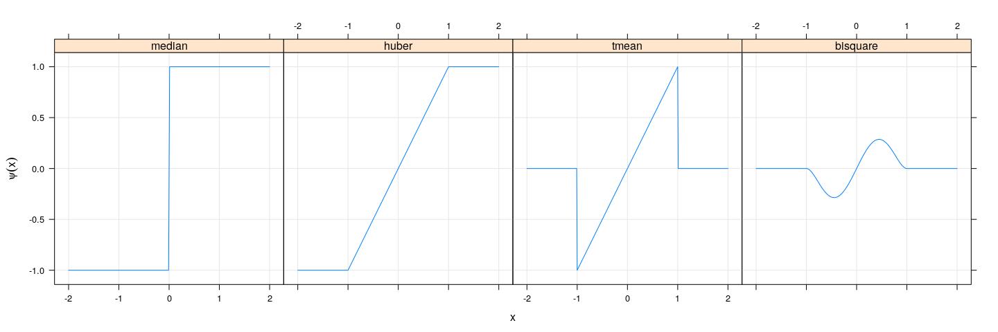
Common robust loss function derivatives
xx <- seq(-2, 2, 0.01)
c <- 1; R <- 1
psi <-
    data.frame(xx = xx,
               median = sign(xx),
               huber = ifelse(abs(xx) <= c, xx, c * sign(xx)),
               tmean = ifelse(abs(xx) <= c, xx, 0),
               bisquare = xx * pmax(0, (1 - (xx/R)^2))^2)
xyplot(median + huber + tmean + bisquare ~ xx, psi, type = "l", outer = TRUE,
       ylab = expression(psi(x)), xlab = "x", grid = TRUE)
![plot of chunk unnamed-chunk-13]()
Common robust loss function derivatives
The last two functions are examples of “redescending” influence functions
Corresponding loss function \(\rho\) becomes flat beyond a threshold
In effect, beyond this threshold, extreme observations are completely discounted
In other words, they have zero/constant contribution to the total loss
However, this does make the objective function (to be minimized) non-convex
- Let us see what the objective function looks like for various loss functions
huber.loss <- function(x, c = 1) ifelse(abs(x) < c, x^2, c * (2 * abs(x) - c))
bisquare.loss <- function(x, R = 1) ifelse(abs(x) < R, R^2 * (1 - (1 - (x/R)^2))^3, R^2)
x <- rnorm(10)
y <- c(x, 10.1, 10.2, 10.3) # add three extreme observations to x
t <- seq(-5, 15, 0.01)
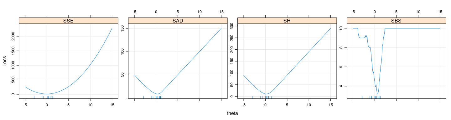
Example: loss functions
SSE <- sapply(t, function(theta) sum((x - theta)^2))
SAD <- sapply(t, function(theta) sum(abs(x - theta)))
SH <- sapply(t, function(theta) sum(huber.loss(x - theta, c = 1)))
SBS <- sapply(t, function(theta) sum(bisquare.loss(x - theta, R = 1)))
xyplot(SSE + SAD + SH + SBS ~ t, type = "l", outer = TRUE,
       ylab = "Loss", xlab = "theta", grid = TRUE, scales = list(y = "free")) +
    layer(panel.rug(x = .GlobalEnv$x))
![plot of chunk unnamed-chunk-15]()
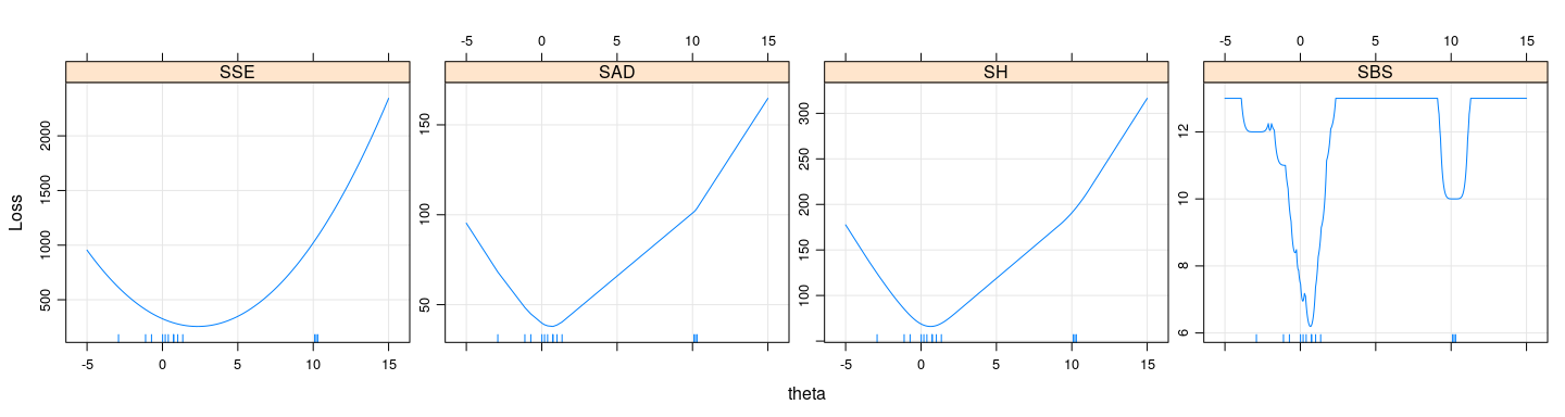
Example: loss functions
SSE <- sapply(t, function(theta) sum((y - theta)^2))
SAD <- sapply(t, function(theta) sum(abs(y - theta)))
SH <- sapply(t, function(theta) sum(huber.loss(y - theta, c = 1)))
SBS <- sapply(t, function(theta) sum(bisquare.loss(y - theta, R = 1)))
xyplot(SSE + SAD + SH + SBS ~ t, type = "l", outer = TRUE,
       ylab = "Loss", xlab = "theta", grid = TRUE, scales = list(y = "free")) +
    layer(panel.rug(x = .GlobalEnv$y))
![plot of chunk unnamed-chunk-16]()
- For non-convex loss functions, important to have good starting estimates
Other practical considerations
Tuning parameters are arbitrary
Natural to express tuning parameter in terms of scale \(\sigma\) (unknown) — scale invariance
Common to take \(\hat\sigma\) to be a multiple of the median absolute deviation (MAD) from the median
Tuning parameter can then be chosen to achieve some target asymptotic relative efficiency under normality
For example, Huber loss function with \(c = 1.345 \sigma\) would give 95% \(ARE\) if \(\sigma\) was known
Standard errors
- M-estimators are consistent and asymptotically normal with variance \(\tau \sigma^2 / n\), where
\[
\tau = \frac{E(\psi^2(X))}{ [ E(\psi^{\prime}(X)) ]^2 }
\]
- Could be estimated by replacing \(X\) by fitted (standardized) residuals
\[
\hat\tau = \frac{\frac{1}{n} \sum_i \psi^2(e_i / \hat\sigma)}{ [ \frac{1}{n} \sum_i \psi^{\prime}(e_i / \hat\sigma) ]^2 }
\]
- Not necessarily reliable in small samples
M-estimation for regression
The ideas described above translate directly to linear regression
Instead of minimizing least squared errors, minimize
\[
\sum_{i=1}^n \rho(y_i - \mathbf{x}_i^T \beta)
\]
- Simple estimation approach: Iteratively (Re)Weighted Least Squares (IWLS / IRLS) with weights
\[
w_i^{(t+1)} = \frac{\psi\left(y_i - \mathbf{x}_i^T \hat{\beta}^{(t)}\right)}
{y_i - \mathbf{x}_i^T \hat{\beta}^{(t)}} =
\frac{\psi(e_i^{(t)})}{e_i^{(t)}} > 0
\]
Implemented in the rlm() function (in the MASS package) among others
By default, scale is estimated using MAD of residuals (updated for each iteration)
M-estimation example: Bisquare
![plot of chunk unnamed-chunk-17]()
M-estimation example: Huber
![plot of chunk unnamed-chunk-18]()
M-estimation example: Least absolute deviation (using optim())
![plot of chunk unnamed-chunk-19]()
M-estimation example: multiple regression
              Estimate Std. Error   t value     Pr(>|t|)
(Intercept) -6.0646629 4.27194117 -1.419650 1.630896e-01
income       0.5987328 0.11966735  5.003310 1.053184e-05
education    0.5458339 0.09825264  5.555412 1.727192e-06
                 Value Std. Error   t value
(Intercept) -7.4121192 3.87702087 -1.911808
income       0.7902166 0.10860468  7.276082
education    0.4185775 0.08916966  4.694169
                 Value Std. Error   t value
(Intercept) -7.1107028 3.88131509 -1.832034
income       0.7014493 0.10872497  6.451593
education    0.4854390 0.08926842  5.437970
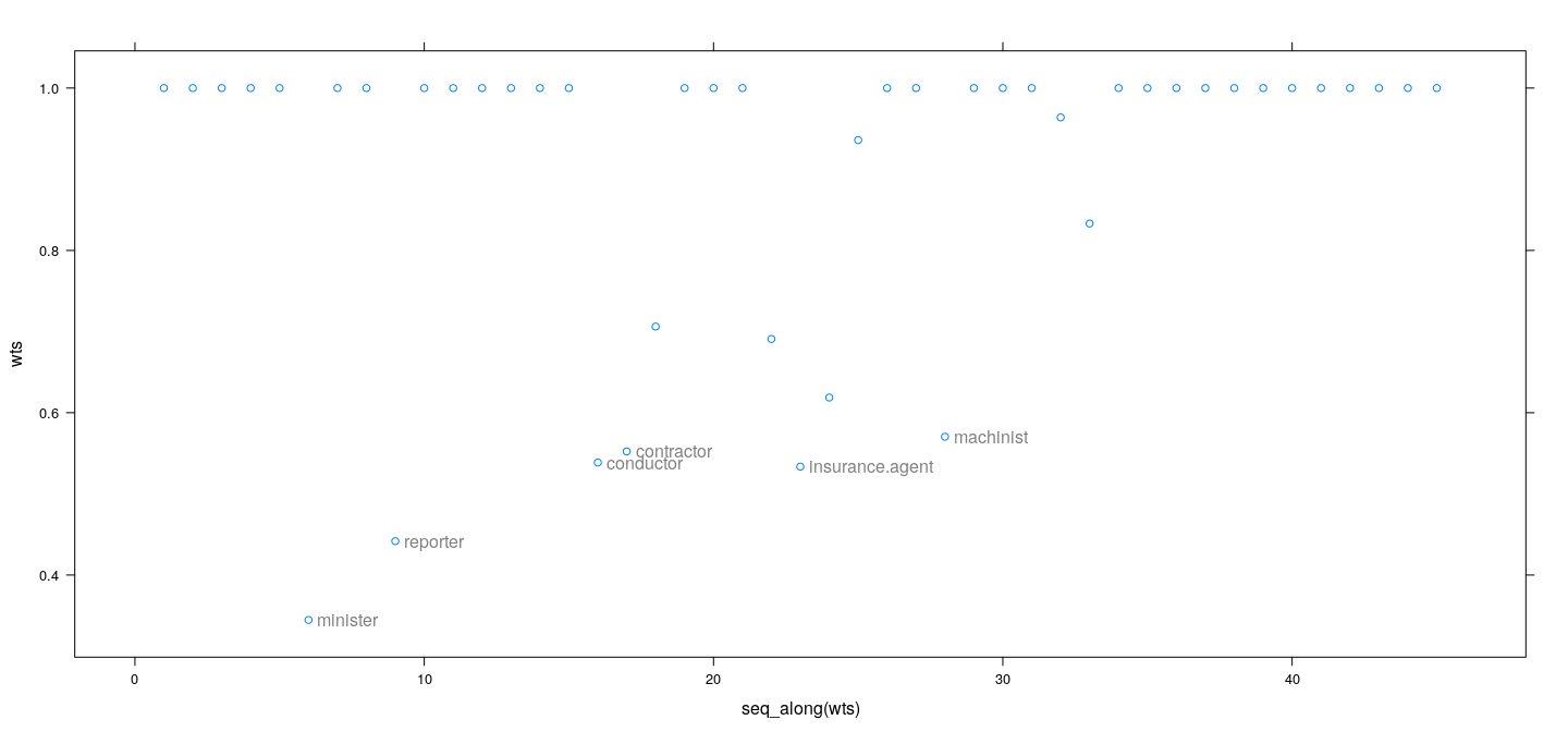
M-estimation example: weights as diagnostics
- IWLS weights give an alternative measure of influence
![plot of chunk unnamed-chunk-21]()
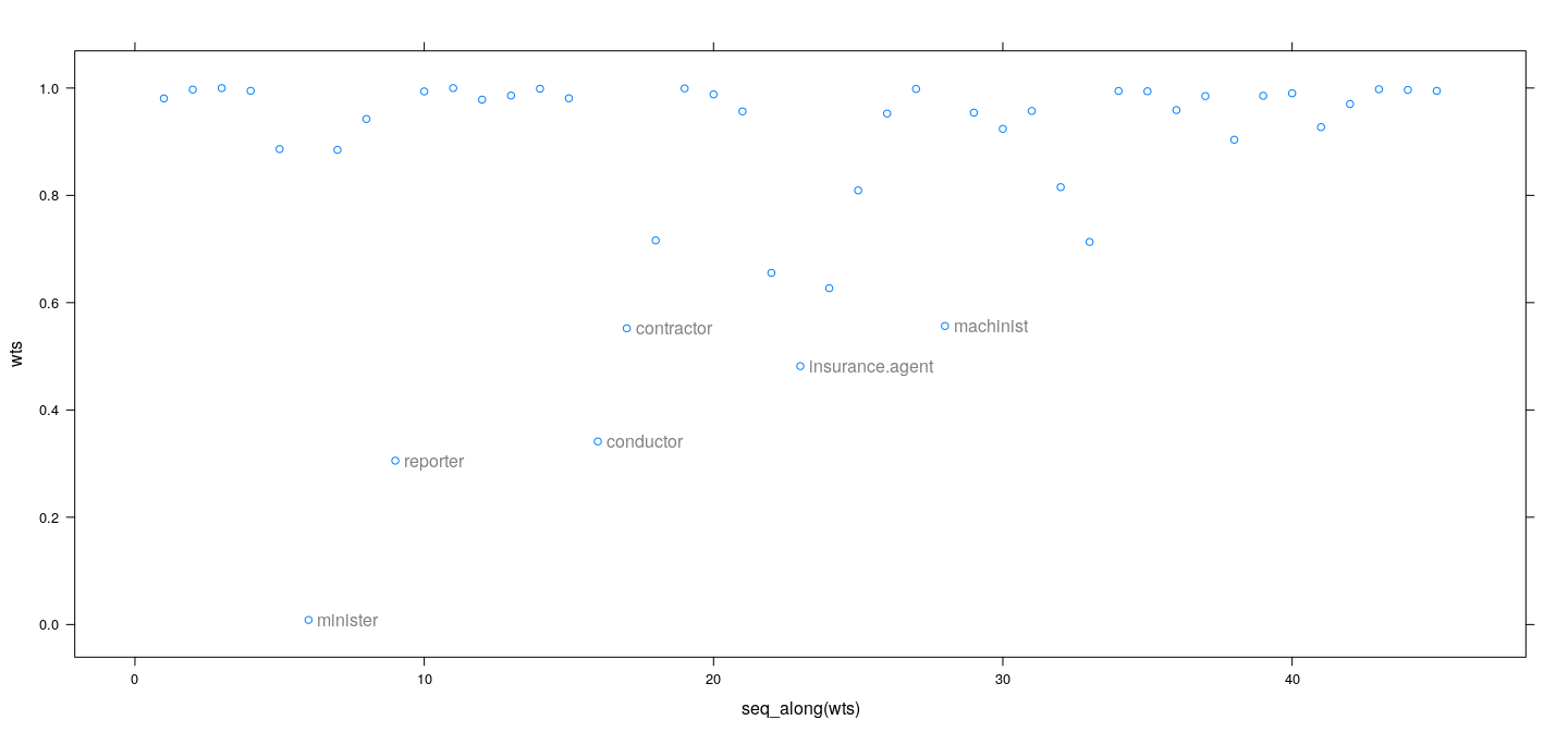
M-estimation example: weights as diagnostics
- IWLS weights give an alternative measure of influence
![plot of chunk unnamed-chunk-22]()
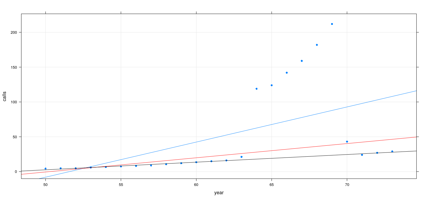
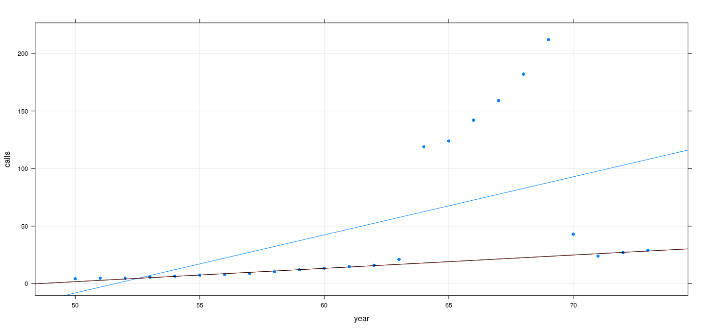
Does M-estimation ensure high breakdown point?
Example: Number of phone calls (in millions) in Belgium
Data available in the MASS package
For 1964–1969, length of calls (in minutes) had been recorded instead of number
Does M-estimation ensure high breakdown point?
data(phones, package = "MASS")
fm2 <- rlm(calls ~ year, data = phones, psi = psi.huber, maxit = 100)
fm3 <- rlm(calls ~ year, data = phones, psi = psi.bisquare)
xyplot(calls ~ year, data = phones, grid = TRUE, type = c("p", "r"), pch = 16) +
    layer(panel.abline(fm2, col = "red")) + layer(panel.abline(fm3, col = "black"))
![plot of chunk unnamed-chunk-23]()
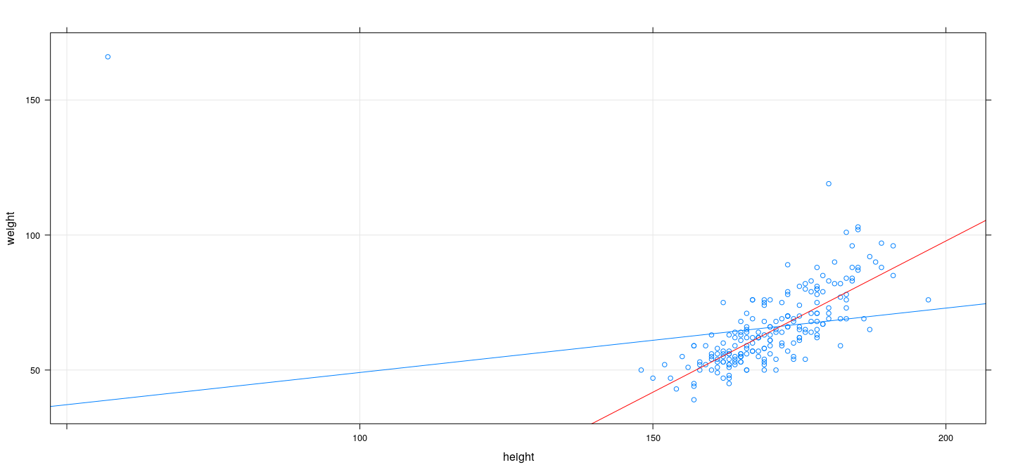
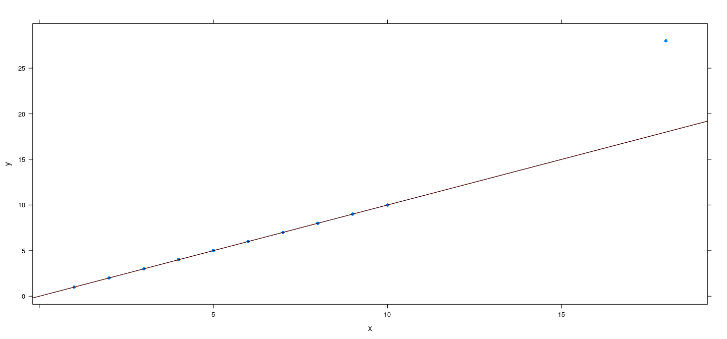
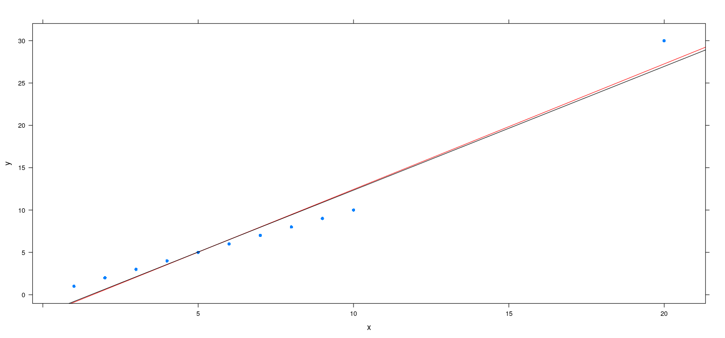
An artificial example
![plot of chunk unnamed-chunk-24]()
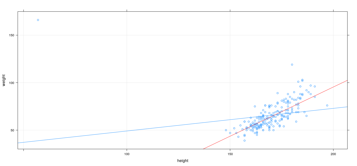
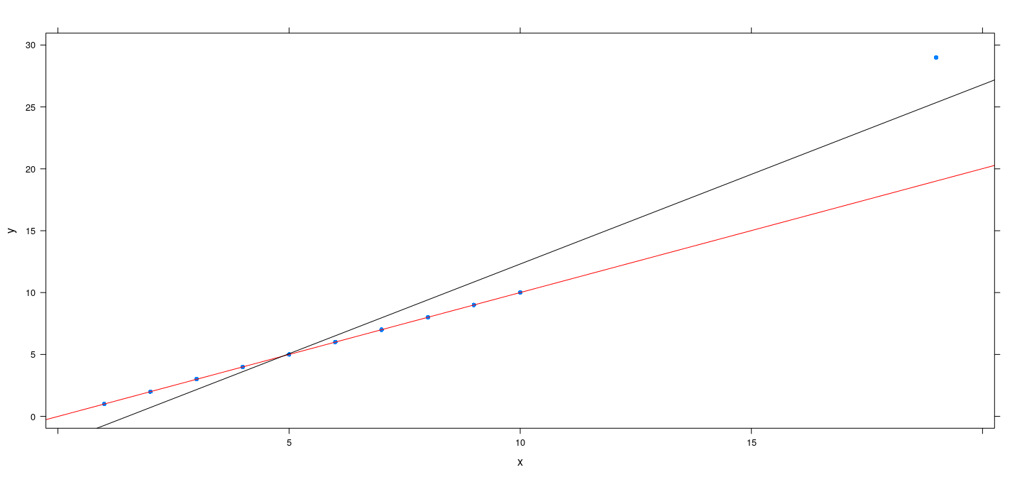
An artificial example
![plot of chunk unnamed-chunk-25]()
An artificial example
![plot of chunk unnamed-chunk-26]()
Why does this happen?
M-estimation approach can ensure high breakdown point for univariate location estimation
This is not automatically true for regression
Increasing loss function (LAD, Huber): sufficiently high-leverage outlier can always attract optimum line
Loss functions that flatten out (Bisquare): result depends on choice of \(c\) (which is estimated)
In general, no guarantee that M-estimation approach has bounded influence in regression
Resistant regression
Resistant alternatives exist, but are much more difficult to fit computationally
We will mention two examples: LMS and LTS regression
Least Median of Squares (LMS) regression: Find \(\hat{\beta}\) as
\[
\arg \min_\beta \mathrm{median}\left\lbrace (y_i - \mathbf{x}_i^T \beta)^2 ; i = 1, \dotsc, n\right\rbrace
\]
More generally, LQS minimizes some quantile of the squared errors
Least Trimmed Squares (LTS) regression: Find \(\hat{\beta}\) as
\[
\arg \min_\beta \sum_{i=1}^q (y_i - \mathbf{x}_i^T \beta)^2_{(i)}
\]
Resistant regression: LMS and LTS
Both LMS/LQS and LTS have high resistance (breakdown point) but low efficiency
LMS/LQS has lower efficiency than LTS, and there is no reason to prefer LMS over LTS
Computation of both are difficult
The MASS package provides one implementation in lmsreg() and ltsreg()
Example: Number of phone calls (in millions) in Belgium
data(phones, package = "MASS")
fm2 <- lmsreg(calls ~ year, data = phones)
fm3 <- ltsreg(calls ~ year, data = phones)
xyplot(calls ~ year, data = phones, grid = TRUE, type = c("p", "r"), pch = 16) +
    layer(panel.abline(fm2, col = "red")) + layer(panel.abline(fm3, col = "black"))
![plot of chunk unnamed-chunk-27]()
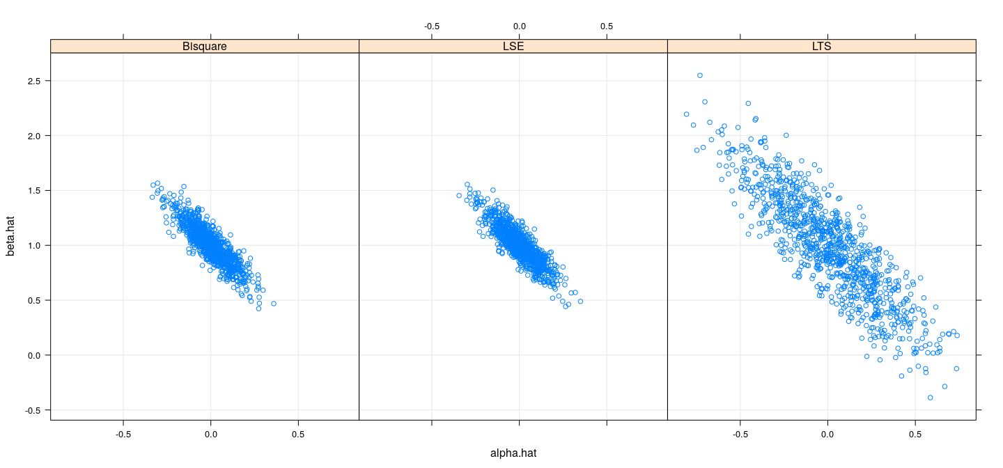
Efficiency comparison: simulation study (normal)
simulateCoefN <- function(n)
{
    x <- runif(n, 0, 1)
    y <- x + 0.5 * rnorm(n)
    fm1 <- lm(y ~ x)
    fm2 <- rlm(y ~ x, psi = psi.bisquare)
    fm3 <- ltsreg(y ~ x)
    data.frame(rbind(coef(fm1), coef(fm2), coef(fm3)),
               model = c("LSE", "Bisquare", "LTS"))
}
sim.coefsn <- replicate(1000, simulateCoefN(100), simplify = FALSE)
sim.coefsn.df <- do.call(rbind, sim.coefsn)
names(sim.coefsn.df) <- c("alpha.hat", "beta.hat", "model")
Efficiency comparison: simulation study (normal)
![plot of chunk unnamed-chunk-29]()
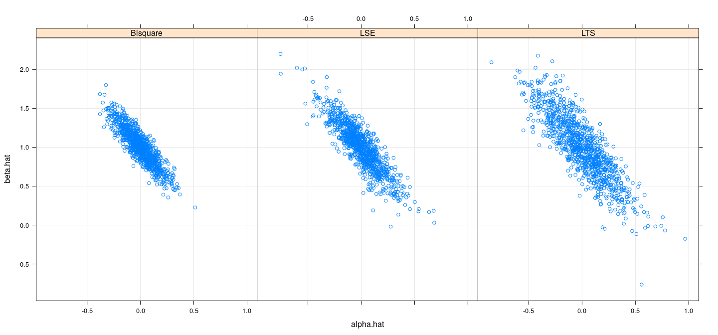
Efficiency comparison: simulation study (\(t_3\))
simulateCoefT <- function(n)
{
    x <- runif(n, 0, 1)
    y <- x + 0.5 * rt(n, df = 3)
    fm1 <- lm(y ~ x)
    fm2 <- rlm(y ~ x, psi = psi.bisquare)
    fm3 <- ltsreg(y ~ x)
    data.frame(rbind(coef(fm1), coef(fm2), coef(fm3)),
               model = c("LSE", "Bisquare", "LTS"))
}
sim.coefst <- replicate(1000, simulateCoefT(100), simplify = FALSE)
sim.coefst.df <- do.call(rbind, sim.coefst)
names(sim.coefst.df) <- c("alpha.hat", "beta.hat", "model")
Efficiency comparison: simulation study (\(t_3\))
![plot of chunk unnamed-chunk-31]()
MM-estimation
M-estimation with Bisquare error has reasonable efficiency
Should have high breakdown point if scale is “correctly” estimated
High breakdown potentially fails if initial scale estimate is too high
MM-estimation tries to ensure high breakdown point with high efficiency of Bisquare loss
First step is to obtain a better scale estimate using S-estimation (will not discuss)
This is followed by M-estimation with Bisquare loss function calibrated by estimated scale
Implemented in rlm() with method = "MM"
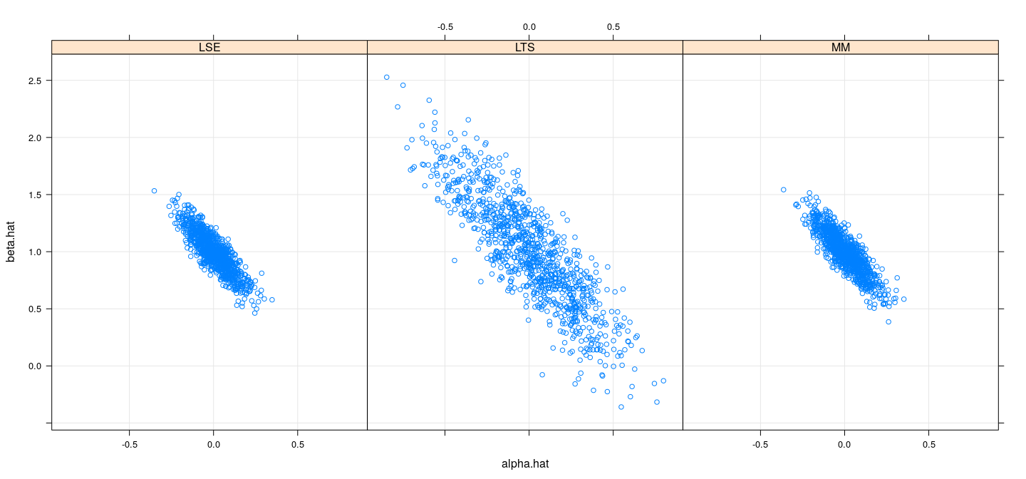
Efficiency comparison: simulation study (normal)
simulateCoefMM <- function(n)
{
    x <- runif(n, 0, 1)
    y <- x + 0.5 * rnorm(n)
    fm1 <- lm(y ~ x)
    fm2 <- rlm(y ~ x, method = "MM")
    fm3 <- ltsreg(y ~ x)
    data.frame(rbind(coef(fm1), coef(fm2), coef(fm3)),
               model = c("LSE", "MM", "LTS"))
}
sim.coefsmm <- replicate(1000, simulateCoefMM(100), simplify = FALSE)
sim.coefsmm.df <- do.call(rbind, sim.coefsmm)
names(sim.coefsmm.df) <- c("alpha.hat", "beta.hat", "model")
Efficiency comparison: simulation study (normal)
![plot of chunk unnamed-chunk-33]()
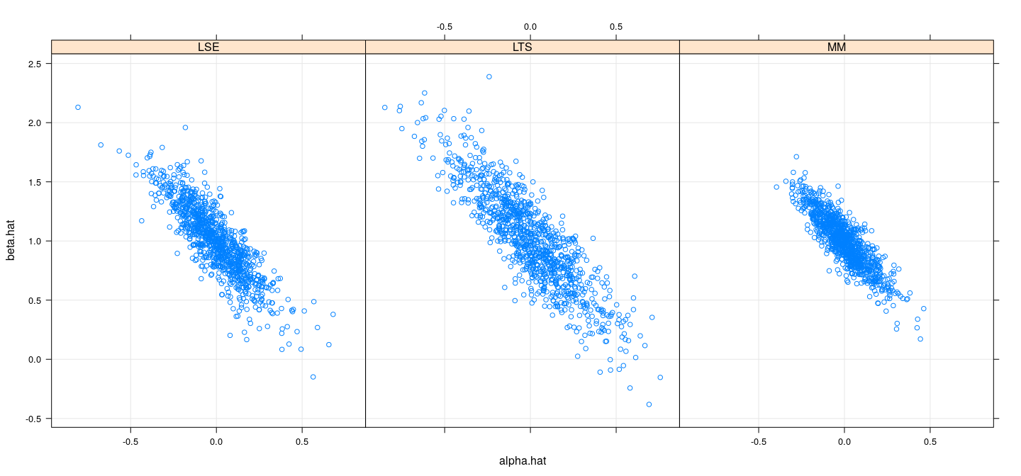
Efficiency comparison: simulation study (\(t_3\))
simulateCoefMMt <- function(n)
{
    x <- runif(n, 0, 1)
    y <- x + 0.5 * rt(n, df = 3)
    fm1 <- lm(y ~ x)
    fm2 <- rlm(y ~ x, method = "MM")
    fm3 <- ltsreg(y ~ x)
    data.frame(rbind(coef(fm1), coef(fm2), coef(fm3)),
               model = c("LSE", "MM", "LTS"))
}
sim.coefsmmt <- replicate(1000, simulateCoefMMt(100), simplify = FALSE)
sim.coefsmmt.df <- do.call(rbind, sim.coefsmmt)
names(sim.coefsmmt.df) <- c("alpha.hat", "beta.hat", "model")
Efficiency comparison: simulation study (\(t_3\))
![plot of chunk unnamed-chunk-35]()
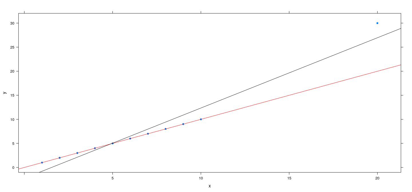
Artificial example revisited
![plot of chunk unnamed-chunk-36]()
Software implementations in R