Unusual and Influential Observations
Deepayan Sarkar
Violation of assumptions in a linear regression model
Systematic violations
- Non-normality of errors
- Nonconstant error variance
- Lack of fit (nonlinearity)
- Autocorrelation in errors
Discordant outliers and influential observations
For now, we will focus on indentifying such observations
Violation of assumptions in a linear regression model
- Outline
- Motivation and description of diagnostic measures
- Cutoffs for diagnostics (mostly heuristic)
- Mathematical details
- References
- Cook and Weisberg (1982) Residuals and influence in regression.
- Belsley, Kuh, Welsh (1980) Regression diagnostics: Identifying influential data and sources of collinearity
- Chatterjee and Hadi (1988) Sensitivity analysis in linear regression
Important concepts
- Regression Outlier : Conditional distribution of \(Y_i|X_i\) is unusual (discrepancy)
![plot of chunk unnamed-chunk-1]()
Important concepts
- Covariate Outlier : \(X_i\) value is unusual w.r.t. other values of \(X\) (may also be a regression outlier)
![plot of chunk unnamed-chunk-2]()
Important concepts
- Leverage : Potential ability of an observation to affect (influence) regression
![plot of chunk unnamed-chunk-3]()
Important concepts
- Leverage : Potential ability of an observation to affect (influence) regression
![plot of chunk unnamed-chunk-4]()
Important concepts
- Leverage : Potential ability of an observation to affect (influence) regression
![plot of chunk unnamed-chunk-5]()
General principle: outliers, leverage, and influence
Covariate outliers have high leverage (potentially influential)
Whether a discrepant observation (regression outlier) actually influences fit depends on whether it also has high leverage
Roughly, influence = leverage \(\times\) discrepancy
We want to be able to identify high-leverage observations, regression outliers, and influential observations
Relatively simple for single predictor, but want general methods that work with many predictors
Leverage: hat-values
In the linear model, \(\hat\beta\) is a linear function of \(\mathbf{y}\):
\[
\hat\beta = (\mathbf{X}^T \mathbf{X})^{-1} \mathbf{X}^T \mathbf{y}
\]
So is the vector of fitted values:
\[
\hat{\mathbf{y}} = \mathbf{X} \hat\beta = \mathbf{X} (\mathbf{X}^T \mathbf{X})^{-1} \mathbf{X}^T \mathbf{y} = \mathbf{H} \mathbf{y}
\]
where \(\mathbf{H} = \mathbf{X} (\mathbf{X}^T \mathbf{X})^{-1} \mathbf{X}^T\) is known as the “hat matrix”
Leverage: hat-values
In scalar notation,
\[
\hat{y_j} = \sum_{i=1}^n h_{ji} y_i = \sum_{i=1}^n h_{ij} y_i
\]
\(h_{ij}\)-s depend on \(\mathbf{X}\), not \(\mathbf{y}\)
\(h_{ij}\) captures contribution of \(y_i\) on \(\hat{y_j}\) (larger values means potentially larger impact)
Hat-values (summarize leverage of \(y_i\) on all fitted values):
\[
h_i \equiv h_{ii} = \sum_{j=1}^n h^2_{ij}
\]
The last result follows because \(\mathbf{H}\) is symmetric and idempotent (\(\mathbf{H}^2 = \mathbf{H}\))
Corollary: \(V(\hat{\mathbf{y}}) = \sigma^2 \mathbf{H}\) and \(V(\hat{\mathbf{e}}) = \sigma^2 (\mathbf{I} - \mathbf{H})\), where \(e_i = y_i - \hat{y}_i\)
Properties of hat-values \(h_i\)
\(0 \leq h_i \leq 1\)
- In fact, \(h_i \geq 1/n\) if the model includes the constant term
- Easy to check if other columns are orthogonal to \(\mathbf{1}\) (mean zero)
- Enough to verify that \(\mathbf{H}\) remains unchanged (exercise)
- \(\bar{h} = p/n\) where \(p\) is the rank of \(\mathbf{X}\)
- Proof follows from property of idempotent / projection matrices: rank = trace
Properties of hat-values \(h_i\)
For simple linear regression with one predictor, \(h_i\) simplifies to
\[
h_i = \frac{1}{n} + \frac{(x_i - \bar{x})^2}{\sum_j (x_j - \bar{x})^2}
\]
In general, with \(\tilde{\mathbf{X}}\) denoting “centered” \(\mathbf{X}\) (mean zero columns),
\[
h_i = \frac{1}{n} + \tilde{\mathbf{x}}_i^T ( \tilde{\mathbf{X}}^T
\tilde{\mathbf{X}} )^{-1} \tilde{\mathbf{x}}_i
\]
So \(h_i\) essentially measures (up to scaling) the Mahalanobis distance of \(\mathbf{x}_i\) from the centroid (mean vector) of the covariates (taking their correlation structure into account)
Properties of hat-values \(h_i\)
![plot of chunk unnamed-chunk-6]()
Properties of hat-values \(h_i\)
fm <- lm(prestige ~ education + income, Duncan, na.action = na.exclude)
id <- which(hatvalues(fm) > 0.15)
levelplot(hatvalues(fm) ~ education + income, Duncan, main = "Hat-values", cex = 1.5,
          panel = panel.levelplot.points, prepanel = prepanel.default.xyplot) +
    layer(panel.text(x[id], y[id], labels = rownames(Duncan)[id], pos = 4, col = "grey50"))
![plot of chunk unnamed-chunk-7]()
Detecting outliers: standardized and Studentized residuals
Regression outliers have high discrepancy, i.e., high \(\varepsilon_i\)
Unfortunately, corresponding \(\hat{\varepsilon}_i\) may not be large
As noted earlier, \(V(e_i) = \sigma^2 (1 - h_i)\)
Define standardized residual :
\[
r_i = \frac{e_i}{\hat\sigma \sqrt{1-h_i}}
\]
Unfortunately, numerator and denominator are not independent.
Deletion models
\[
t_i = \frac{e_i}{\hat\sigma_{(-i)} \sqrt{1-h_i}}
\]
- May be more natural to define the deleted Studentized residual
\[
\tilde{t}_i = \frac{e_{i(-i)}}{\hat{V} (e_{i(-i)}) }
\]
- \(\hat{V} (e_{i(-i)})\) needs to be computed, but involves unknown \(\sigma\), which is replaced by \(\hat\sigma_{(-i)}\)
Testing for outliers in linear models
\(t_i\) can be used to test if observation \(i\) is an outlier
Makes sense if we suspected that the \(i\)th observation was an outlier
Usually we don’t know in advance, and want to test for all \(i\)
This leads to a multiple testing situation
Expect \(\alpha n\) tests to be rejected even if no outliers (assuming independent tests)
Testing for outliers in linear models: usual strategies
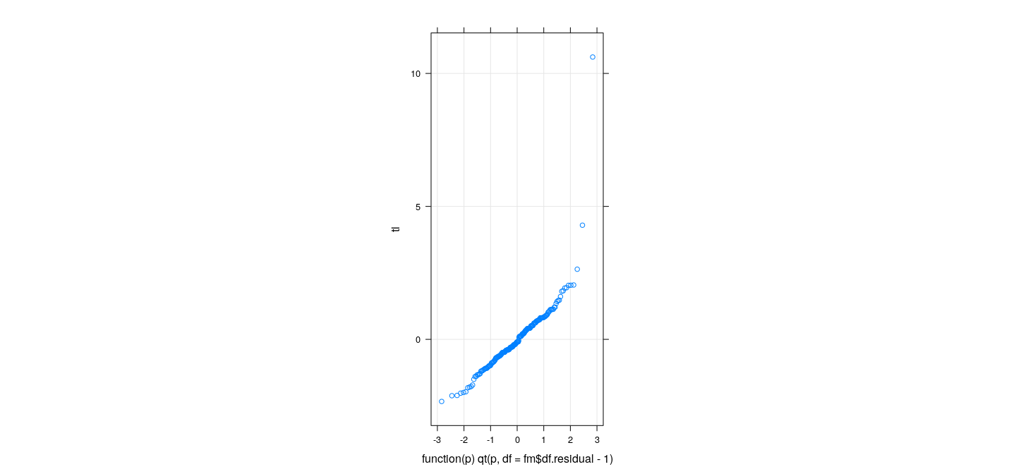
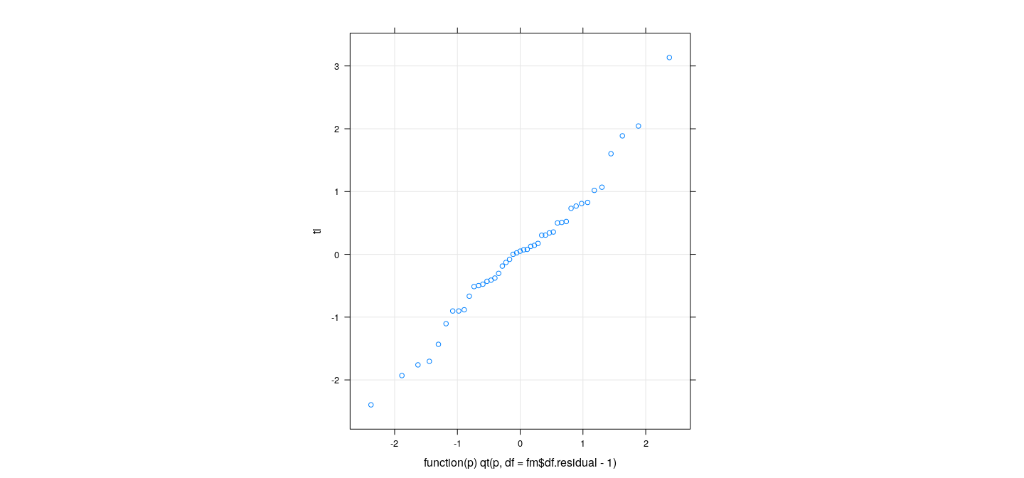
Examine graphically (Q-Q plot comparing to \(t_{n-p-1}\))
Simulate the largest (absolute) \(t_i\) from the null model (distribution does not depend on \(\beta\) or \(\sigma^2\) — exercise)
If we assume independence, the smallest \(p\)-value has a Beta distribution
- \(p\)-values are all independent \(U(0,1)\) under null
- Interested in the distribution of the smallest of these, follows Beta\((1, n)\)
- CDF easily computed as \(F(u) = 1 - (1-u)^n\)
Testing for outliers in linear models: usual strategies
\[
P(\text{at least one rejection}) = P\left(\cup \{np_i < \alpha\}\right) \leq \sum P\left(p_i < \frac{\alpha}{n}\right) \leq \sum \frac{\alpha}{n} = n \frac{\alpha}{n} = \alpha
\]
Testing for outliers in linear models: usual strategies
Both these procedures can be viewed as an adjustment to the original \(p\)-values
Test \(i\) is rejected if the adjusted \(p_i\) is less than \(\alpha\)
The Bonferroni adjustment is \(p^{\prime}_i = n p_i\)
Adjustment with independent tests is \(p^{\prime}_i = 1 - (1 - p_i)^n\)
p.adjust() implements various \(p\)-value adjustment procedures in R
Testing for outliers: examples
![plot of chunk unnamed-chunk-9]()
Testing for outliers: examples
[1] "12" "21"
[1] "12" "21"
[1] "12" "21"
Testing for outliers: examples
![plot of chunk unnamed-chunk-11]()
Testing for outliers: examples
character(0)
character(0)
character(0)
       minister        reporter      contractor insurance.agent       machinist     store.clerk
    0.003177202     0.021170298     0.047432955     0.060427645     0.066248120     0.085783008
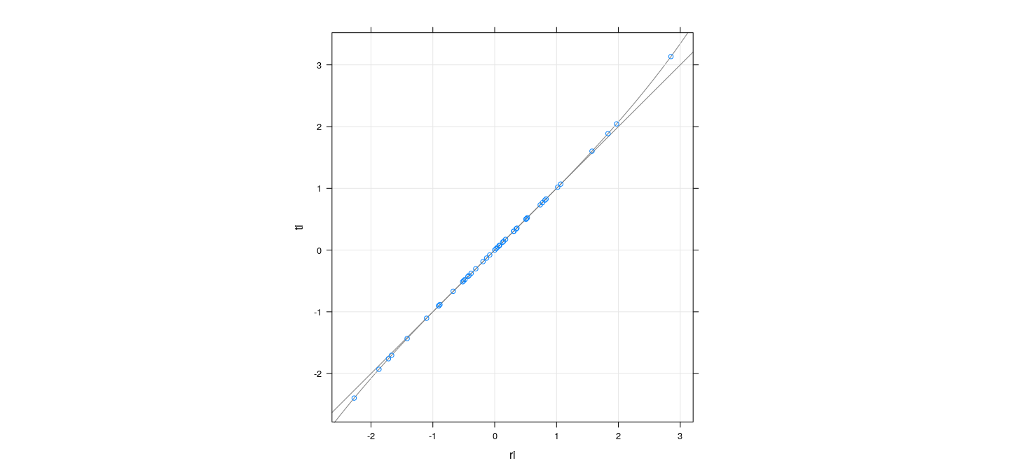
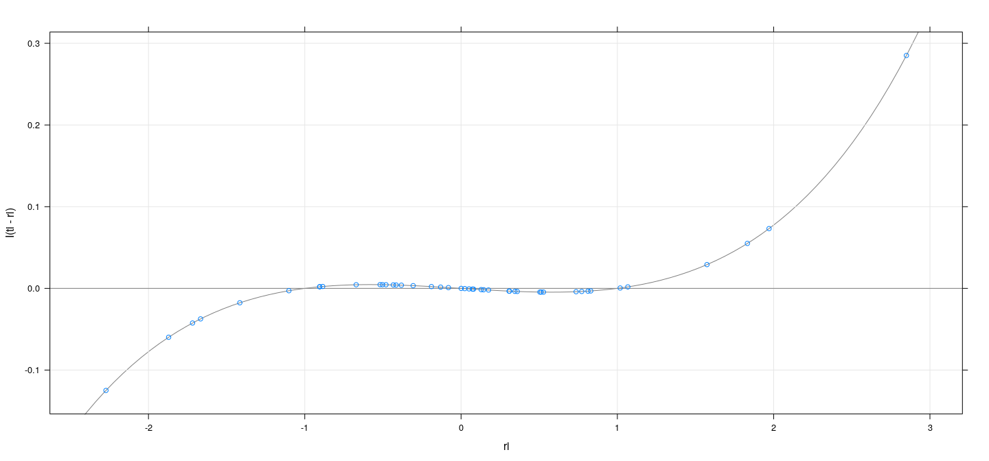
A useful relationship
As already noted, \(e_{i(-i)} = e_i / (1 - h_i)\)
This means that to compute \(e_{i(-i)}\), we do not actually need to re-fit model
In particular, leave-one-out cross-validation SSE can be calculated without actually re-fitting models
- There is a similar exact relationship between \(r_i\) and \(t_i\)
\[
t_i = r_i \sqrt{\frac{n-p-1}{n-p-r_i^2}}
\]
A useful relationship
![plot of chunk unnamed-chunk-14]()
A useful relationship
![plot of chunk unnamed-chunk-15]()
Measures of influence
We are typically more interested in influential observations
Direct measure of the influence of objervation \(i\) on coefficient \(\beta_j\) is (for \(i = 1, \dotsc, n; j = 1, \dotsc, p\))
\[
DFBETA_{ij} = d_{ij} = \hat{\beta}_j - \hat{\beta}_{j(-i)}
\]
- It is common to standardize this:
\[
DFBETAS_{ij} = d^{*}_{ij} = \frac{d_{ij}}{SE_{(-i)}(\hat{\beta}_j)}
\]
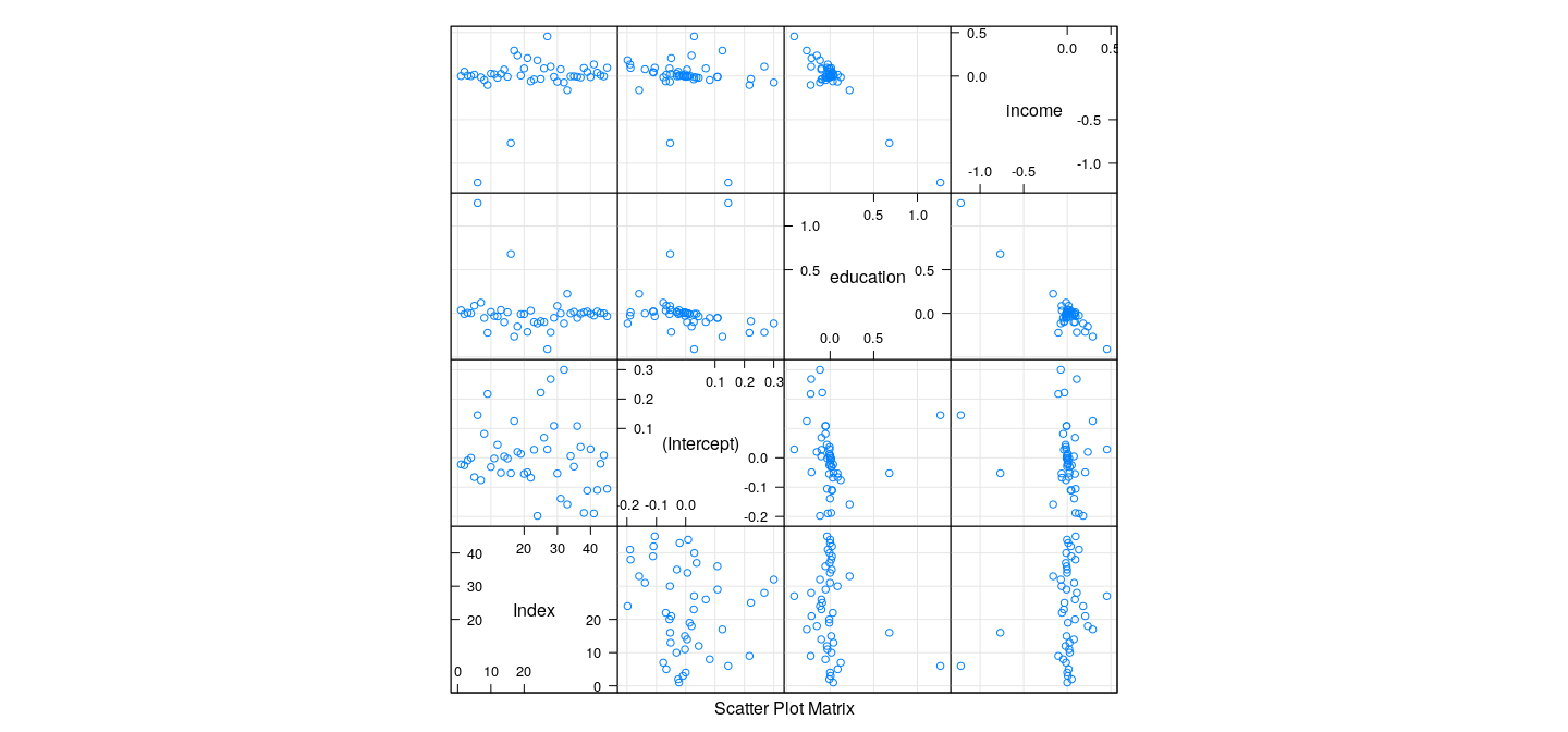
Drawback: there can be many of them (\(np\) in total).
When \(p\) is small, it is useful to plot \(DFBETA_{ij}\) (or \(DFBETAS_{ij}\)) against \(i\) separately for each \(j\).
It is also common to look at a summary influence measure for each observation.
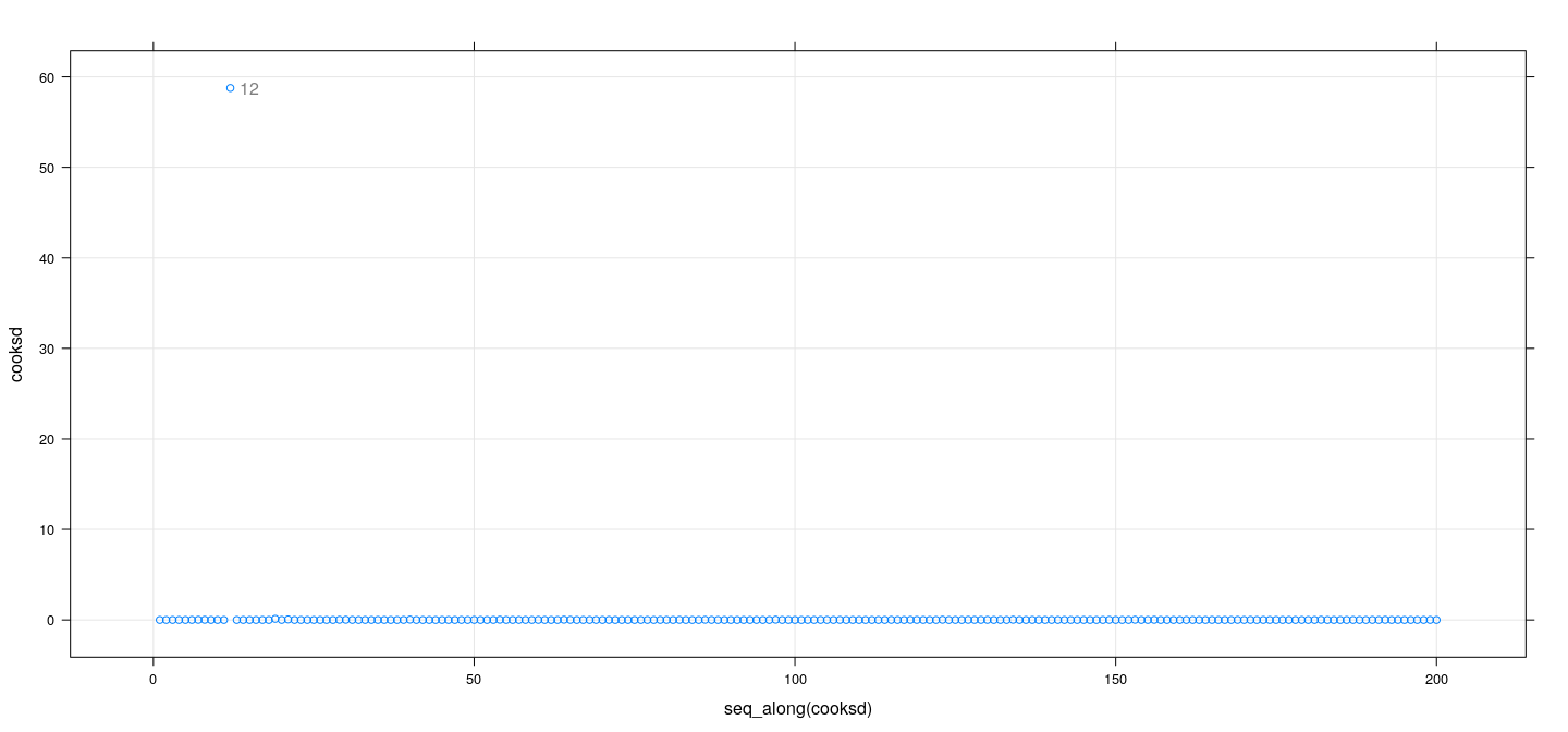
Cook’s distance
Think of testing the “hypothesis” that \(\beta = \hat{\beta}_{(-i)}\)
Consider the “\(F\)-statistic” for this test, recalculated for each \(i\) (though not really meaningful)
This is known as Cook’s distance \(D_i\). It can be shown that
\[
D_i = \frac{{r_i}^2}{p} \times \frac{h_i}{1-h_i}
\]
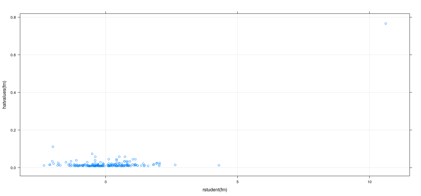
DFFITS
\[
DFFITS_i = t_i \times \sqrt{\frac{h_i}{1-h_i}}
\]
- In most cases (since \(t_i \approx r_i\))
\[
D_i \approx \frac{DFFITS_i^2}{p}
\]
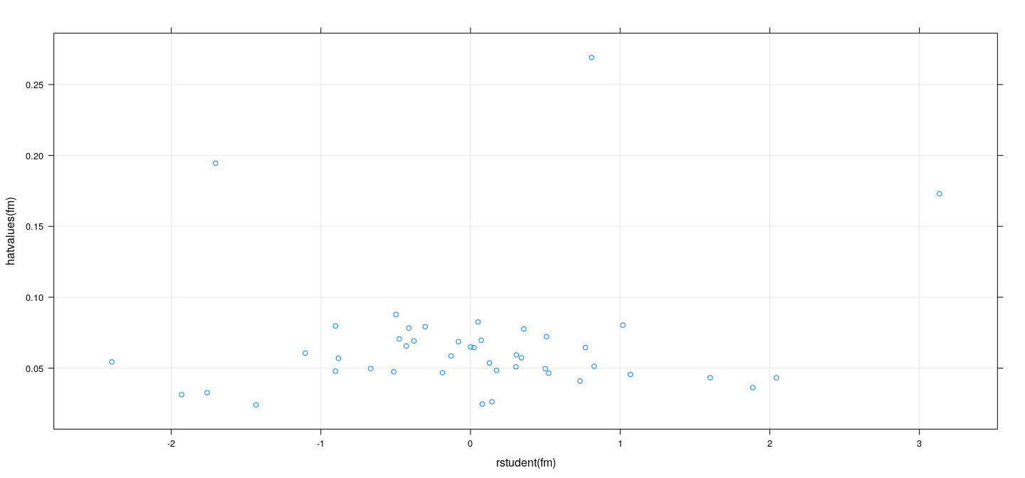
- A graphical alternative is to plot \(h_i\) vs \(t_i\) and look for unusual extreme values.
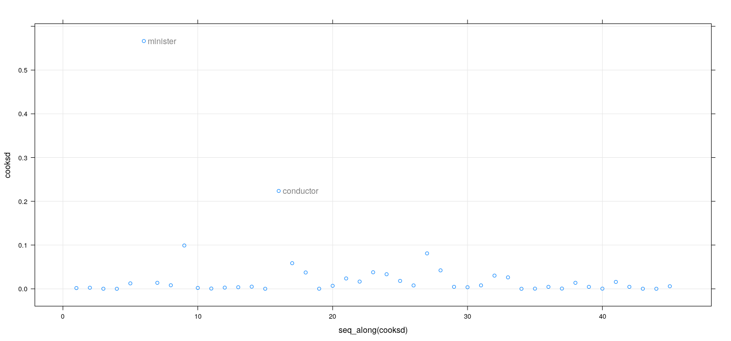
Measures of influence: examples
![plot of chunk unnamed-chunk-16]()
Measures of influence: examples
![plot of chunk unnamed-chunk-17]()
Measures of influence: examples
![plot of chunk unnamed-chunk-18]()
Measures of influence: examples
![plot of chunk unnamed-chunk-19]()
Measures of influence: examples
![plot of chunk unnamed-chunk-20]()
Influence on standard errors
Individual observations can also influence standard errors
For example, standard error for estimated slope in simple linear regression \(y = \alpha + \beta x + \varepsilon\)
\[
s.e.(\hat{\beta}) = \frac{\hat{\sigma}}{\sqrt{\sum_i (x_i - \bar{x})^2}}
\]
- High leverage + low discrepancy: may decrease standard error without influencing estimated coefficients
Influence on standard errors
Generally, we could measure influence by effect on size of joint confidence region of \(\hat{\beta}\)
Measure proposed by Belsley et al (1980)
\[\begin{eqnarray*}
COVRATIO_i &=& \frac{ \lvert \hat{\sigma}^2_{(-i)} (\mathbf{X}^T \mathbf{X})^{-1}_{(-i)} \rvert } { \lvert \hat{\sigma}^2 (\mathbf{X}^T \mathbf{X})^{-1} \rvert } \\
&=& \frac{1}{ (1-h_i) } \times \left( \frac{\hat{\sigma}^2_{(-i)}}{\hat{\sigma}^2} \right)^p = \frac{1}{ (1-h_i) \left( \frac{n-p-1 + t^2_i}{n-p} \right)^p }
\end{eqnarray*}\]
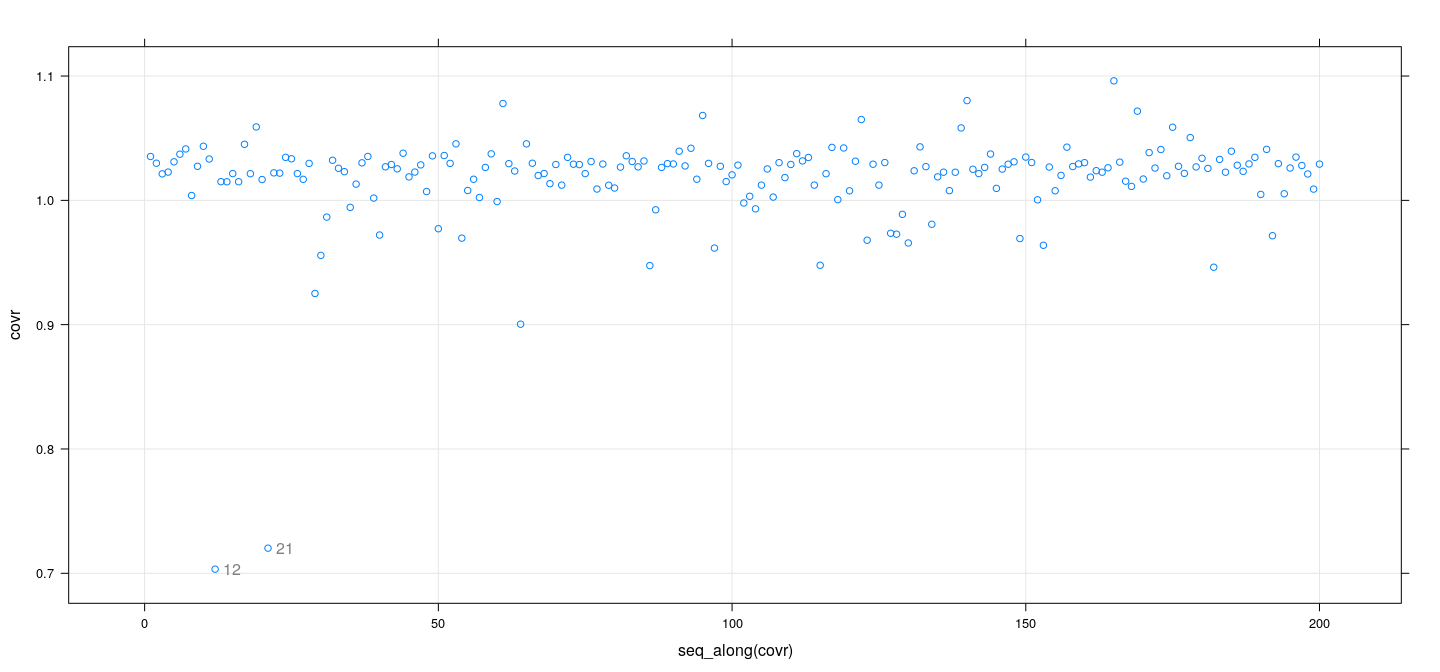
Observations that increase precision have \(COVRATIO_i > 1\)
Observations that decrease precision have \(COVRATIO_i < 1\)
Look for values that differ from 1
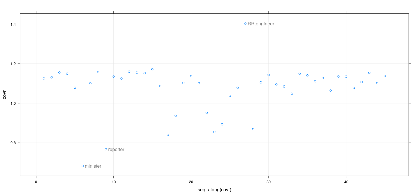
Measures of influence: examples
![plot of chunk unnamed-chunk-22]()
Measures of influence: examples
![plot of chunk unnamed-chunk-23]()
Numerical cutoffs
Blindly following numerical cutoffs is not recommended
Most regression diagnostics are designed for graphical examination
Still, numerical cutoffs can be a useful complement
Particularly useful to indicate a “cutoff line” on a graph
Numerical cutoffs
Hat values: \(2 \times \frac{p}{n}\) or \(3 \times \frac{p}{n}\) for small samples
Studentized residuals: \(\pm 2\) (adjusted \(p\)-value for more formal test)
- \(DFBETAS_{ij}\)
- As these are standardized, an absolute cutoff of 1 or 2 is reasonable
- For large \(n\), a size adjusted cutoff \(2 / \sqrt{n}\) is suggested by Belsley et al
Cook’s distance \(D\): analogy with \(F\)-test gives a natural cutoff (Chatterjee and Hadi, 1988)
\[
D_i > \frac{4}{n-p}
\]
- Translates to cutoff for \(DFFITS\) using approximate relation with \(D_i\)
\[
DFFITS_i > 2 \sqrt{ \frac{p}{n-p} }
\]
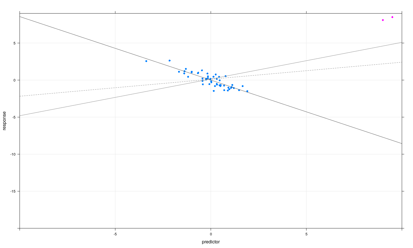
Jointly influential observations
- Subsets of observations can be jointly influential, or can offset each other
![plot of chunk unnamed-chunk-24]()
Jointly influential observations
- Subsets of observations can be jointly influential, or can offset each other
![plot of chunk unnamed-chunk-25]()
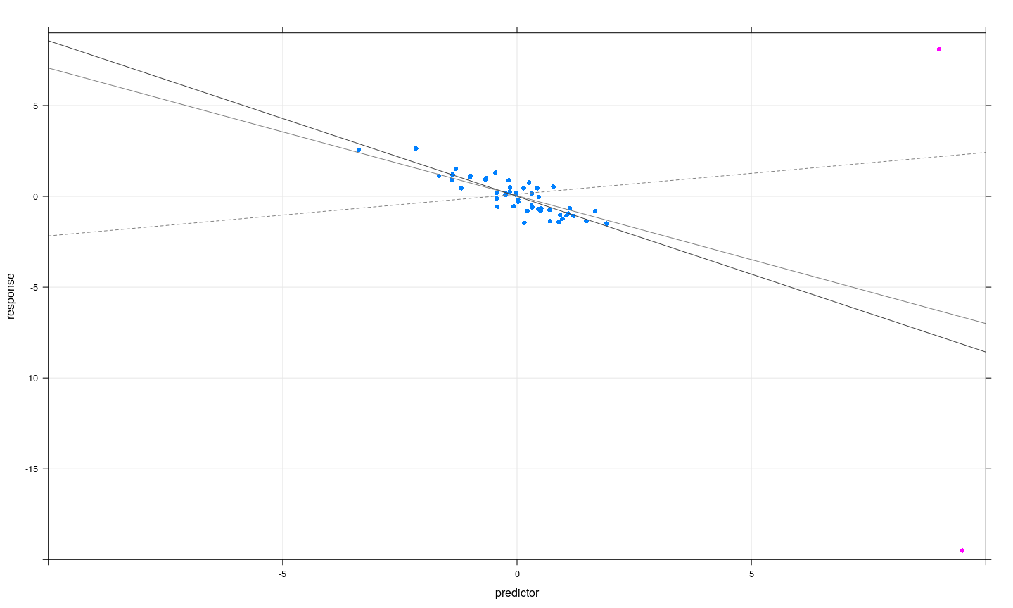
Jointly influential observations
- Subsets of observations can be jointly influential, or can offset each other
![plot of chunk unnamed-chunk-26]()
Jointly influential observations: possible strategies
Find most influential observation
If considered unusual, remove, re-fit model, and consider next most influential observation
Can often work, but is not always successful
Alternatively, extend Cook’s distance to subsets of observations
Number of possible subsets can become large
Graphical alternative: partial regression / added variable plots
Insight: Jointly influential observations easy to detect visually for single covariate
Can we reduce multiple regression to simple regression?
Partial regression plots can do this, provided we focus on influence on one coefficient at a time
Partial regression
Question: What is the interpretation of \(\beta_j\) in the Mutiple regression model
\[
\mathbf{y} = \beta_0 \mathbf{1} + \beta_1 \mathbf{x}^{(1)} + \cdots + \beta_j \mathbf{x}^{(j)} + \cdots + \beta_p \mathbf{x}^{(p)}
\]
(where \(\mathbf{x}^{(j)}\) represents \(j\)-th column of \(\mathbf{X}\))
\(\beta_j\) is effect of \(j\)-th covariate \(x^{(j)}\) on response \(y\)
\(t\)-test for \(\beta_j = 0\) tests significance of \(\beta_j\) in the presence of other covariates
Significance determined by amount of reduction in total sum of squares
Partial regression: example
[1] 27493.32
(Intercept)      height        dsex
109.1141967  -0.3129827  22.4980107
(Intercept)      height
 25.2662278   0.2384059
Partial regression: example
Can we recover the additional effect of \(\beta_j\) from the partial model?
[1] 33166.05
(Intercept)        dsex
  -6.436995   14.629534
Partial regression: example
Can we recover the additional effect of \(\beta_j\) from the partial model?
[1] 27493.32
residuals(lm(dsex ~ 1 + height))
                        22.49801
Partial regression / added variable plot for \(\beta_j\)
Denote \(\mathbf{X}\) excluding its \(j\)-th column by \(\mathbf{X}^{(-j)}\)
Regress \(\mathbf{y}\) on \(\mathbf{X}^{(-j)}\), denote residual vector by \(\mathbf{y}^{(j)}\)
Regress \(j\)-th column of \(\mathbf{X}\) on \(\mathbf{X}^{(-j)}\), denote residual vector by \(\mathbf{X}^{(j)}\)
In other words
Plot \(\mathbf{y}^{(j)}\) against \(\mathbf{X}^{(j)}\)
This is useful because the coefficient of this regression is the same as \(\hat{\beta}_j\)
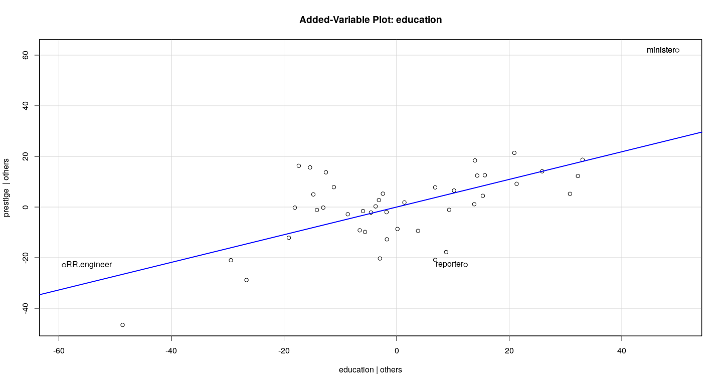
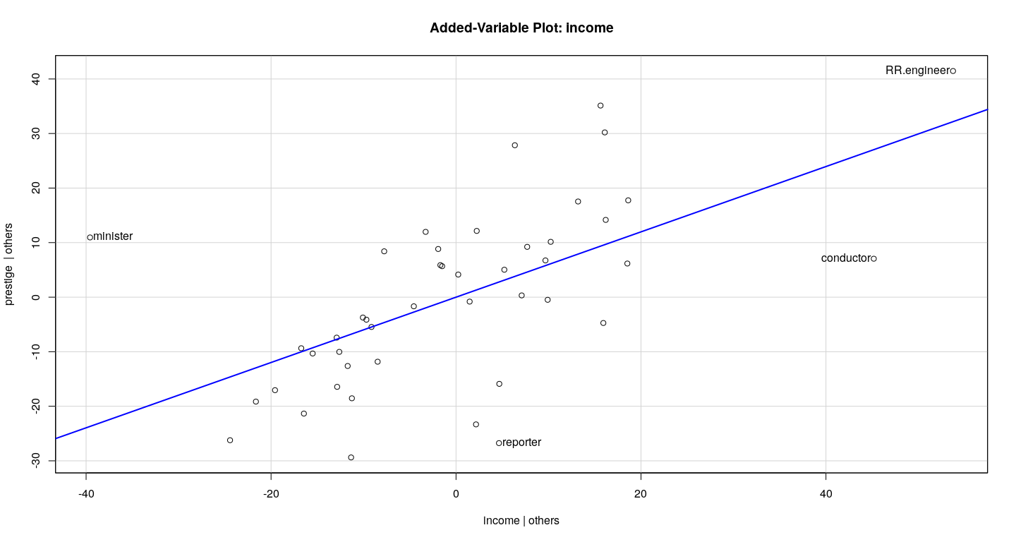
Example: Duncan data
![plot of chunk unnamed-chunk-29]()
Example: Duncan data
![plot of chunk unnamed-chunk-30]()
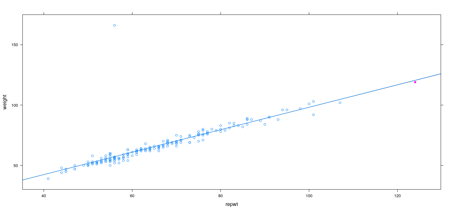
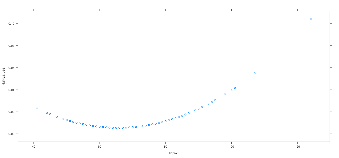
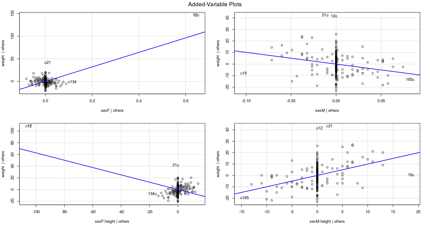
Example: Davis data
![plot of chunk unnamed-chunk-31]()
What should we do with unusual data?
Easy solution: discard
This is sometimes the right thing to do, but should not be done automatically
Unusual data may provide insight (e.g., Duncan’s prestige data)
It may indicate data recording errors (e.g., Davis data has values switched)
   sex weight height repwt repht
10   M     65    171    64   170
11   M     70    175    75   174
12   F    166     57    56   163
13   F     51    161    52   158
14   F     64    168    64   165
- Finally, can try alternatives to least squares: robust regression