An Overview of the R Programming Environment

R for Clinical Trials

What is R?

• An environment for statistical computing and graphics (from website)

• Available as Free / Open Source Software

• Very popular (both academia and industry)

• Easy to try out on your own

Is it suitable for clinical trials research / analysis?

• Yes! See this Task View if you are looking for specific methods not covered in the workshop

• For regulatory issues, see the R certification page

• Ask me if you still have any concerns after this workshop

Is R better than SAS?

• I don’t know SAS, so I don’t have an opinion

• Both are tools, you should use what you are comfortable with

Main differences: (from looking at some SAS examples for this workshop)

• R is designed to be used interactively

• It is more similar to traditional programming languages like C / Java / Python

• Almost everything in R is done by calling functions (similar to SAS PROCs?)

• Writing new functions is much easier (and very common) in R

Overall agenda for the workshop

• Informal overview of R

• More formal introduction to the language

• Statistical analyis (model fitting, visualization, tests)

• Case studies using clinical trial examples

Outline of first part: Overview

• Installing R

• Basics of using R

• Example: Linear regresion

• Working with “reproducible documents”

Installing R

• R is most commonly used as a REPL (Read-Eval-Print-Loop)

  • When it is started, R Waits for user input

  • Evaluates and prints result

  • Waits for more input

• There are several different interfaces to do this

• R itself works on many platforms (Windows, Mac, UNIX, Linux)

• Some interfaces are platform-specific, some work on most

• R and the interface may need to be installed separately

• I assume you have already done this! Otherwise:

• Go to https://cran.r-project.org/ (or choose a mirror first)

• Follow instructions depending on your platform (probably Windows)

• This will install R, as well as a default graphical interface on Windows and Mac

• I recommend a different interface called R Studio that needs to be installed separately

• I hope that you have also done this (but it is not essential)

Running R

• Once installed, you can start the appropriate interface (or R directly) to get something like this:

R Under development (unstable) (2019-12-29 r77627) -- "Unsuffered Consequences"
Copyright (C) 2019 The R Foundation for Statistical Computing
Platform: x86_64-pc-linux-gnu (64-bit)

R is free software and comes with ABSOLUTELY NO WARRANTY.
You are welcome to redistribute it under certain conditions.
Type 'license()' or 'licence()' for distribution details.

  Natural language support but running in an English locale

R is a collaborative project with many contributors.
Type 'contributors()' for more information and
'citation()' on how to cite R or R packages in publications.

Type 'demo()' for some demos, 'help()' for on-line help, or
'help.start()' for an HTML browser interface to help.
Type 'q()' to quit R.

Loading required package: utils
> 

• The > represents a prompt indicating that R is waiting for input.

• The difficult part is to learn what to do next

The R REPL essentially works like a calculator

34 * 23

[1] 782

27 / 7

[1] 3.857143

exp(2)

[1] 7.389056

2^10

[1] 1024

• Formally, R evaluates the expression typed in at the prompt

• This may sometimes result in an error (or a + prompt requesting more input)

R has standard mathematical functions

sqrt(5 * 125)

[1] 25

log(120)

[1] 4.787492

factorial(10)

[1] 3628800

log(factorial(10))

[1] 15.10441

Most non-trivial tasks involve calling functions

choose(15, 5)

[1] 3003

factorial(15) / (factorial(10) * factorial(5))

[1] 3003

choose(1500, 2)

[1] 1124250

factorial(1500) / (factorial(1498) * factorial(2))

[1] NaN

R supports variables

x <- 2
y <- 10
x^y

[1] 1024

y^x

[1] 100

factorial(y)

[1] 3628800

log(factorial(y), base = 10)

[1] 6.559763

Variable assignment is done using “ a <- b ” , but “ a = b ” also works

R can compute on vectors

N <- 15
x <- seq(0, N)
N

[1] 15

x

 [1]  0  1  2  3  4  5  6  7  8  9 10 11 12 13 14 15

choose(N, x)

 [1]    1   15  105  455 1365 3003 5005 6435 6435 5005 3003 1365  455  105   15    1

This is one of the most important distinguishing features of R

R has built-in functions for probability calculations

p <- 0.25
choose(N, x) * p^x * (1-p)^(N-x)

 [1] 1.336346e-02 6.681731e-02 1.559070e-01 2.251991e-01 2.251991e-01 1.651460e-01 9.174777e-02 3.932047e-02
 [9] 1.310682e-02 3.398065e-03 6.796131e-04 1.029717e-04 1.144130e-05 8.800998e-07 4.190952e-08 9.313226e-10

dbinom(x, size = N, prob = p)

 [1] 1.336346e-02 6.681731e-02 1.559070e-01 2.251991e-01 2.251991e-01 1.651460e-01 9.174777e-02 3.932047e-02
 [9] 1.310682e-02 3.398065e-03 6.796131e-04 1.029717e-04 1.144130e-05 8.800998e-07 4.190952e-08 9.313226e-10

• The results of any evaluation is usually printed, unless assigned to a variable

• When printing vectors, R prefixes each output line with the index of the first element

R has functions that work on vectors

p.x <- dbinom(x, size = N, prob = p)
sum(x * p.x) / sum(p.x)

[1] 3.75

N * p

[1] 3.75

R can draw graphs

plot(x, p.x, ylab = "Probability", pch = 16)
title(main = sprintf("Binomial(%g, %g)", N, p))
abline(h = 0, col = "grey")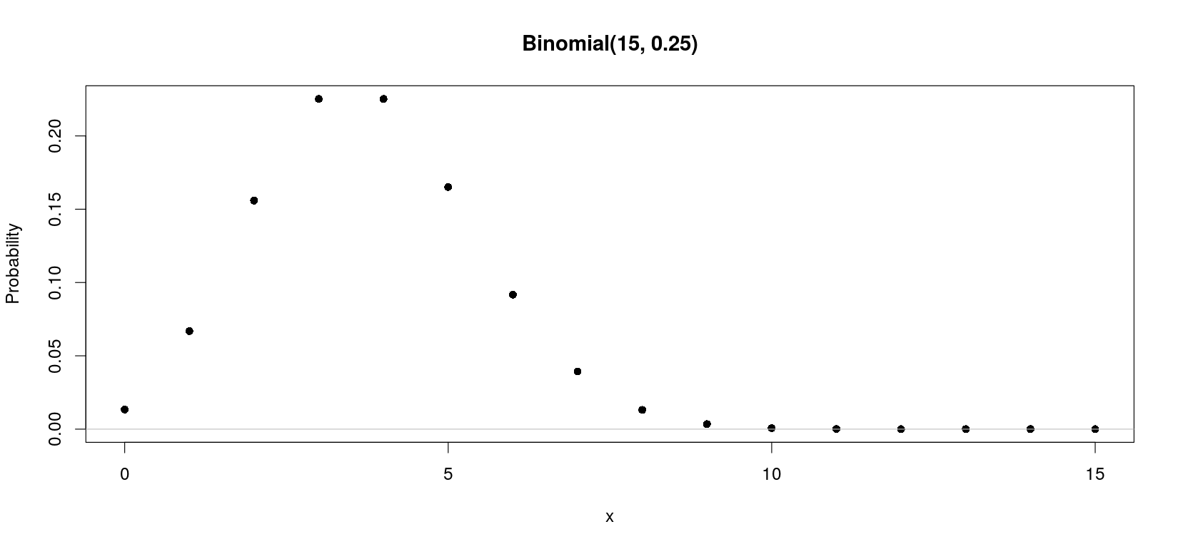

R can simulate random variables

cards <- as.vector(outer(c("H", "D", "C", "S"), 1:13, paste))
cards

 [1] "H 1"  "D 1"  "C 1"  "S 1"  "H 2"  "D 2"  "C 2"  "S 2"  "H 3"  "D 3"  "C 3"  "S 3"  "H 4"  "D 4"  "C 4" 
[16] "S 4"  "H 5"  "D 5"  "C 5"  "S 5"  "H 6"  "D 6"  "C 6"  "S 6"  "H 7"  "D 7"  "C 7"  "S 7"  "H 8"  "D 8" 
[31] "C 8"  "S 8"  "H 9"  "D 9"  "C 9"  "S 9"  "H 10" "D 10" "C 10" "S 10" "H 11" "D 11" "C 11" "S 11" "H 12"
[46] "D 12" "C 12" "S 12" "H 13" "D 13" "C 13" "S 13"

sample(cards, 13)

 [1] "H 2"  "H 6"  "S 2"  "C 12" "D 11" "H 4"  "D 1"  "C 9"  "C 4"  "H 5"  "C 11" "D 3"  "C 7" 

sample(cards, 13)

 [1] "H 9"  "H 1"  "H 2"  "C 8"  "C 12" "S 6"  "S 5"  "S 4"  "S 12" "C 10" "H 8"  "C 9"  "D 1" 

z <- rnorm(50, mean = 0, sd = 1)
z

 [1]  0.3719275  0.1936631  0.9836552 -0.4919062 -1.7152266 -0.9536651  0.9155696  1.5895887 -0.3702185
[10]  0.9767307 -1.1981943  0.6387483 -0.8821841 -1.3193350 -0.2383257  0.1816948  0.7416892  0.3211718
[19] -0.8479021 -0.4725004  0.6577830  1.4740185  1.3978639 -0.9053331 -1.3183413 -0.4472865  0.9149328
[28]  0.6456813 -0.2279315  0.4666840  0.5562906  1.9223093 -2.4408218 -1.0598998 -1.5190523 -0.4563874
[37]  0.2832823 -1.2485320  0.5840814 -2.1556053 -0.0695510  0.8110716 -1.9551105 -0.8455179  1.0413871
[46] -1.4115850  1.3930437 -0.9093232 -0.2552080  1.2633080

mean(z)

[1] -0.1077754

sd(z)

[1] 1.077932

median(z)

[1] -0.1487413

R is in fact a full programming language

• Variables

• Functions

• Control flow structures

  • For loops, while loops

  • If-then-else (branching)

• Distinguishing features

  • Focus on vectors and vectorized operations

  • Treatment of functions at par with other object types

• We will see a few examples to illustrate what I mean by this

Example: Linear regression

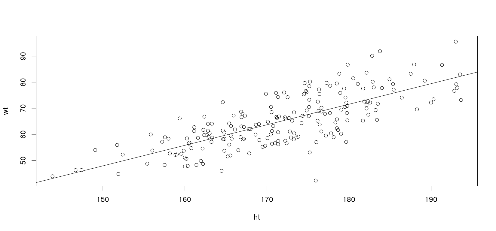
Let us simulate some fake height-weight data

ht <- rnorm(200, mean = 172, sd = 10)    # height in cm
bmi <- rnorm(200, mean = 22, sd = 2.2)   # bmi (independent of height)
wt <- bmi * (ht / 100)^2                 # weight in kg

A simple least squares regression model is fit using the lm() function

fm <- lm(wt ~ ht) # OLS regression of weight on height

As usual, no output is printed is the result is assigned to a variable

Examine fitted model

Useful output is produced by the functions coef() and summary()

coef(fm)

(Intercept)          ht 
-70.1440360   0.7871475 

summary(fm)

Call:
lm(formula = wt ~ ht)

Residuals:
     Min       1Q   Median       3Q      Max 
-26.0490  -4.8284   0.1839   4.5992  17.3154 

Coefficients:
             Estimate Std. Error t value Pr(>|t|)    
(Intercept) -70.14404    8.33442  -8.416 7.73e-15 ***
ht            0.78715    0.04845  16.246  < 2e-16 ***
---
Signif. codes:  0 '***' 0.001 '**' 0.01 '*' 0.05 '.' 0.1 ' ' 1

Residual standard error: 6.744 on 198 degrees of freedom
Multiple R-squared:  0.5714,    Adjusted R-squared:  0.5692 
F-statistic: 263.9 on 1 and 198 DF,  p-value: < 2.2e-16

You should always plot the data to assess model fit!

plot(wt ~ ht)
abline(coef(fm))

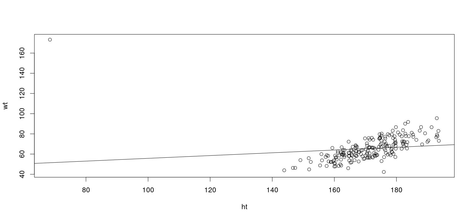
Let’s introduce a mistake in the data

Switch height and weight for the first case

tmp <- wt[1]
wt[1] <- ht[1]
ht[1] <- tmp

Fit the OLS regression line again

fm2 <- lm(wt ~ ht)
summary(fm2)

Call:
lm(formula = wt ~ ht)

Residuals:
    Min      1Q  Median      3Q     Max 
-23.914  -6.989  -1.586   5.451 121.831 

Coefficients:
            Estimate Std. Error t value Pr(>|t|)   
(Intercept) 42.07680   12.61916   3.334  0.00102 **
ht           0.13714    0.07352   1.865  0.06361 . 
---
Signif. codes:  0 '***' 0.001 '**' 0.01 '*' 0.05 '.' 0.1 ' ' 1

Residual standard error: 12.73 on 198 degrees of freedom
Multiple R-squared:  0.01727,   Adjusted R-squared:  0.01231 
F-statistic:  3.48 on 1 and 198 DF,  p-value: 0.06361

Plot the data and regression line again

plot(wt ~ ht)
abline(coef(fm2))

How can we “fix” this?

Two common approaches:

1. Delete “outlier” and re-fit model

2. Use robust regression

   • Least squares fit is sensitive to outliers

   • Instead, minimise sum of absolute errors (or something similar)

How?

• We can find and use a method someone has already implemented

• We can implement a solution of our own

R package ecosystem

• R gives access to an extensive toolset

• Most standard data analysis methods are already implemented

• Can be extended by writing add-on packages

• Thousands of add-on packages are available from CRAN

• Quality varies

• This may matter in regulated environments

For this workshop, I will mostly use the “default” R packages

• These come by default along with a standard installation of R

• Consist of “base” packages

rownames(installed.packages(priority = "base"))

 [1] "base"      "compiler"  "datasets"  "graphics"  "grDevices" "grid"      "methods"   "parallel" 
 [9] "splines"   "stats"     "stats4"    "tcltk"     "tools"     "utils"    

• … and “recommended” packages

rownames(installed.packages(priority = "recommended"))

 [1] "boot"       "class"      "cluster"    "codetools"  "foreign"    "KernSmooth" "lattice"    "MASS"      
 [9] "Matrix"     "mgcv"       "nlme"       "nnet"       "rpart"      "spatial"    "survival"  

There are many other extremely powerful packages that you can explore later

The other option: implement our own solution

• This is often surprisingly easy

• We will come back to the robust regression example later

Interactive vs “pipeline” analysis

R encourages an interactive data analysis workflow

• Result of each step should dictate the next step to take

• Understanding this will help make sense of the design of R

• Sometimes it is useful to apply a standard workflow on a new dataset

• These are usually done using “R scripts”

• I would also strongly encourage using dynamic “notebooks”

Notebooks in R Studio

• Notebooks allow you to mix text and code

• Notebook only contains code, results are dynamically generated

• R Studio supports several variants

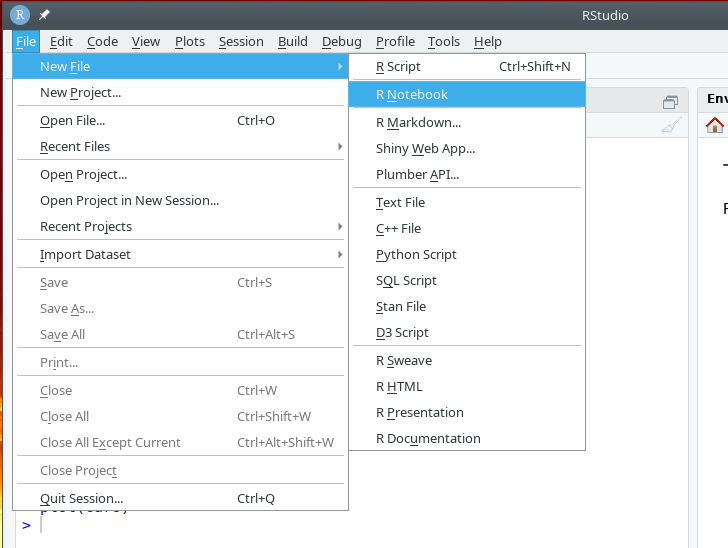
• These slides are written using “R Markdown”

• Open the file names 01-roverview.rmd in R Studio

• These can also be used to generate HTML / PDF / Word reports (requires some more software)

• Benefit: reproducible results, no copy-paste errors

Before we move on…

Please spend some time getting comfortable with R Studio:

• Load the R Markdown file in R Studio

• Run the “code chunks” (marked using ```{r} ... ```)

• Useful shortcut: Ctrl + Shift + Enter

• Try making small changes and re-run