Data manipulation and analysis
Outline
Workflow: multiple datasets and global environment
Variable scope and common “non-standard evaluation” approaches
Data manipulation
Common analysis methods:
- t-test
- ANOVA
- Chi-square test
- Fisher’s exact test
- Kaplan-Meier survival estimates
The global workspace
Variables are symbols associated with some value (technically called a binding)
These symbols are stored in a look-up table
Each variable is stored in a container called an “environment”
Variables defined in an R session are stored in a special environment called the “global environment”
This is also known as the “global workspace”
Let us define some variables in the workspace
treat <- read.table("data/treat-1.txt", header = TRUE, stringsAsFactors = FALSE)
ae <- read.table("data/ae.txt", header = TRUE, stringsAsFactors = FALSE)
str(treat)
'data.frame': 70 obs. of 2 variables:
$ subjid: int 101 102 103 104 105 106 107 108 109 110 ...
$ trtcd : int 1 0 0 1 0 0 1 1 0 1 ...'data.frame': 20 obs. of 5 variables:
$ subjid : int 101 101 102 102 103 103 103 115 115 116 ...
$ aerel : int 1 2 2 1 1 1 2 3 3 2 ...
$ aesev : int 1 1 2 1 1 2 2 2 1 1 ...
$ aebodsys: chr "Cardiac disorders" "Gastrointestinal disorders" "Cardiac disorders" "Psychiatric disorders" ...
$ aedecod : chr "Atrial flutter" "Constipation" "Cardiac failure" "Delirium" ...
Note that the two datasets are connected by a common variable
subjidAdd one more dataset, using the
sas7bdatpackageThis is an experimental package to read files stored in the (undocumented) SAS7BDAT format
library(package = "sas7bdat")
asthma <- read.sas7bdat("sasdata/twosample.sas7bdat")
str(asthma, give.attr = FALSE)
'data.frame': 24 obs. of 4 variables:
$ PATNO: num 101 103 106 108 109 110 113 116 118 120 ...
$ FEV0 : num 1.35 3.22 2.78 2.45 1.84 2.81 1.9 3 2.25 2.86 ...
$ FEV6 : num NaN 3.55 3.15 2.3 2.37 3.2 2.65 3.96 2.97 2.28 ...
$ TRT : Factor w/ 2 levels "ABC-123","PLACEBO": 1 1 1 1 1 1 1 1 1 1 ...- Variables defined in the global workspace can be listed using
ls()
[1] "ae" "asthma" "treat" - But there are clearly many other variables already defined
[1] 3.141593 [1] "Jan" "Feb" "Mar" "Apr" "May" "Jun" "Jul" "Aug" "Sep" "Oct" "Nov" "Dec"
- We can even (apparently) overwrite them
[1] 3.142857[1] "ae" "asthma" "pi" "treat" Other environments and variable scope
R actually looks for variables in several environments sequentially (scope)
The list of these environments, known as the “search path”, is given by
search()
 [1] ".GlobalEnv"        "package:sas7bdat"  "package:lattice"   "package:stats"     "package:graphics"
 [6] "package:grDevices" "package:utils"     "package:datasets"  "package:methods"   "Autoloads"
[11] "package:base"
These environments usually correspond to the various R packages currently loaded
Packages mostly contain functions (which are also bindings) and datasets
A variable is matched to the first occurrence in this list
Possible bindings of a variable can be found using
find()
[1] "package:stats"[1] ".GlobalEnv" "package:base"[1] 3.142857[1] 3.141593Working with datasets
Datasets are also conceptually a collection of variables
It is an attractive idea to make them part of the search path
Error in unique(subjid): object 'subjid' not found [1] ".GlobalEnv" "treat" "package:sas7bdat" "package:lattice" "package:stats"
[6] "package:graphics" "package:grDevices" "package:utils" "package:datasets" "package:methods"
[11] "Autoloads" "package:base" [1] "treat"[1] 70- Unfortunately, this can lead to confusing behaviour
The following object is masked from treat:

subjid [1] ".GlobalEnv" "ae" "treat" "package:sas7bdat" "package:lattice"
[6] "package:stats" "package:graphics" "package:grDevices" "package:utils" "package:datasets"
[11] "package:methods" "Autoloads" "package:base" [1] "ae" "treat"[1] 14- The unpleasant alternative is to qualify each variable by its dataset
[1] 70But this can easily become tedious
Example: t-test comparing FEV1 change (0-6 weeks) by treatment
t.test(x = (asthma$FEV6 - asthma$FEV0)[asthma$TRT == "PLACEBO"],
       y = (asthma$FEV6 - asthma$FEV0)[asthma$TRT == "ABC-123"],
       var.equal = TRUE)
    Two Sample t-test

data:  (asthma$FEV6 - asthma$FEV0)[asthma$TRT == "PLACEBO"] and (asthma$FEV6 - asthma$FEV0)[asthma$TRT == "ABC-123"]
t = -0.97362, df = 19, p-value = 0.3425
alternative hypothesis: true difference in means is not equal to 0
95 percent confidence interval:
 -0.6889311  0.2514766
sample estimates:
mean of x mean of y
0.2840000 0.5027273
Non-standard evaluation
To avoid such tedious use, R offers something known as “non-standard” evaluation
This is an idea that appears in different forms in different functions
The essential idea is that functions are provided a dataset which is temporarily attached during evaluation
General purpose functions:
with()andwithin()Data manipulation functions:
transform(),subset()(see also the popular package dplyr)Used in many contexts: Formula interface (graphics, tests, model fitting)
Basic working knowledge of all these is essential to use R well
The with() function
The simplest of the NSE functions:
with(data, expr)Makes variables in
datatemporarily available in scopeEvaluates the expression given by
exprReturns result of evaluation
with(asthma, t.test(x = (FEV6 - FEV0)[TRT == "PLACEBO"],
                    y = (FEV6 - FEV0)[TRT == "ABC-123"],
                    var.equal = TRUE))
    Two Sample t-test

data:  (FEV6 - FEV0)[TRT == "PLACEBO"] and (FEV6 - FEV0)[TRT == "ABC-123"]
t = -0.97362, df = 19, p-value = 0.3425
alternative hypothesis: true difference in means is not equal to 0
95 percent confidence interval:
 -0.6889311  0.2514766
sample estimates:
mean of x mean of y
0.2840000 0.5027273
Why is this “non-standard” evaluation?
The call is not equivalent to
e <- t.test(x = (FEV6 - FEV0)[TRT == "PLACEBO"],  # gives error
            y = (FEV6 - FEV0)[TRT == "ABC-123"],
            var.equal = TRUE)
with(asthma, e)with()treats itsexprargument as an unevaluated expression
The transform() function
transform()is used to modify or add new variables in a datasetSuppose we want to add a variable
CHGrecording change in FEV1 over the treatment periodWe can do this directly as
- The alternative using
transform()is
'data.frame':   24 obs. of  5 variables:
 $ PATNO: num  101 103 106 108 109 110 113 116 118 120 ...
 $ FEV0 : num  1.35 3.22 2.78 2.45 1.84 2.81 1.9 3 2.25 2.86 ...
 $ FEV6 : num  NaN 3.55 3.15 2.3 2.37 3.2 2.65 3.96 2.97 2.28 ...
 $ TRT  : Factor w/ 2 levels "ABC-123","PLACEBO": 1 1 1 1 1 1 1 1 1 1 ...
 $ CHG  : num  NaN 0.33 0.37 -0.15 0.53 ...
- Note that R functions do not modify their arguments, so the result has to be re-assigned
The within() function
within()is similar, but used for more complex instructionsThe dataset returned contains all modified or newly created variables
within(asthma, # not assigned, so auto-printed ('asthma' remains unchanged)
       {
           FEV6[!is.finite(FEV6)] <- NA # Change NaN to NA
           FEV0[!is.finite(FEV0)] <- NA # Note that CHG, already having NaN, not updated
           PATNO <- as.character(PATNO) # change integer to character
           STRT <- as.character(TRT)    # new variable with treatment as character
       })
PATNO FEV0 FEV6 TRT CHG STRT
1 101 1.35 NA ABC-123 NaN ABC-123
2 103 3.22 3.55 ABC-123 0.33 ABC-123
3 106 2.78 3.15 ABC-123 0.37 ABC-123
4 108 2.45 2.30 ABC-123 -0.15 ABC-123
5 109 1.84 2.37 ABC-123 0.53 ABC-123
6 110 2.81 3.20 ABC-123 0.39 ABC-123
7 113 1.90 2.65 ABC-123 0.75 ABC-123
8 116 3.00 3.96 ABC-123 0.96 ABC-123
9 118 2.25 2.97 ABC-123 0.72 ABC-123
10 120 2.86 2.28 ABC-123 -0.58 ABC-123
11 121 1.56 2.67 ABC-123 1.11 ABC-123
12 124 2.66 3.76 ABC-123 1.10 ABC-123
13 102 3.01 3.90 PLACEBO 0.89 PLACEBO
14 104 2.24 3.01 PLACEBO 0.77 PLACEBO
15 105 2.25 2.47 PLACEBO 0.22 PLACEBO
16 107 1.65 1.99 PLACEBO 0.34 PLACEBO
17 111 1.95 NA PLACEBO NaN PLACEBO
18 112 3.05 3.26 PLACEBO 0.21 PLACEBO
19 114 2.75 2.55 PLACEBO -0.20 PLACEBO
20 115 1.60 2.20 PLACEBO 0.60 PLACEBO
21 117 2.77 2.56 PLACEBO -0.21 PLACEBO
22 119 2.06 2.90 PLACEBO 0.84 PLACEBO
23 122 1.71 NA PLACEBO NaN PLACEBO
24 123 3.54 2.92 PLACEBO -0.62 PLACEBOThe subset() function
- Returns the subset of a dataset containing rows satifying some condition
asthma.placebo <- subset(asthma, TRT == "PLACEBO" & is.finite(CHG))
asthma.abc123 <- subset(asthma, TRT == "ABC-123" & is.finite(CHG))
t.test(asthma.placebo$CHG, asthma.abc123$CHG, var.equal = TRUE)
    Two Sample t-test

data:  asthma.placebo$CHG and asthma.abc123$CHG
t = -0.97362, df = 19, p-value = 0.3425
alternative hypothesis: true difference in means is not equal to 0
95 percent confidence interval:
 -0.6889311  0.2514766
sample estimates:
mean of x mean of y
0.2840000 0.5027273
The split() function
Does not use non-standard evaluation, but extremely useful for data manipulation
Splits one column (or full data frame) into parts by value of one or more categorical columns
Example: split
CHGvariable byTRT
List of 2
 $ ABC-123: num [1:12] NaN 0.33 0.37 -0.15 0.53 ...
 $ PLACEBO: num [1:12] 0.89 0.77 0.22 0.34 NaN 0.21 -0.2 0.6 -0.21 0.84 ...
    Welch Two Sample t-test

data:  PLACEBO and ABC-123
t = -0.97477, df = 18.888, p-value = 0.342
alternative hypothesis: true difference in means is not equal to 0
95 percent confidence interval:
 -0.6885676  0.2511130
sample estimates:
mean of x mean of y
0.2840000 0.5027273
The formula-data interface
A much cleaner alternative to all these is the formula-data interface in
t.test()Such calls usually have a “formula” (containing variable names) and a dataset as the first two arguments
The formula is interpreted in the context of the function
    Welch Two Sample t-test

data:  CHG by TRT
t = 0.97477, df = 18.888, p-value = 0.342
alternative hypothesis: true difference in means is not equal to 0
95 percent confidence interval:
 -0.2511130  0.6885676
sample estimates:
mean in group ABC-123 mean in group PLACEBO
0.5027273 0.2840000 - Let’s revisit the demographic data seen earlier
- Use
within()to convert categorical variables to factors with descriptive labels
demog <- within(demog,
{
    trt = factor(trt, levels = c(1, 0), labels = c("Active", "Placebo"))
    gender = factor(gender, levels = c(1, 2), labels = c("Male", "Female"))
    race = factor(race, levels = c(1, 2, 3), labels = c("White", "Black", "Other"))
})
str(demog)
'data.frame': 60 obs. of 5 variables:
$ subjid: int 101 102 103 104 105 106 201 202 203 204 ...
$ trt : Factor w/ 2 levels "Active","Placebo": 2 1 1 2 1 2 1 2 1 2 ...
$ gender: Factor w/ 2 levels "Male","Female": 1 2 1 2 1 2 1 2 1 2 ...
$ race : Factor w/ 3 levels "White","Black",..: 3 1 2 1 3 1 3 1 2 1 ...
$ age : int 37 65 32 23 44 49 35 50 49 60 ...- Not surprisingly,
t.test()will only work if the right-hand side takes exactly two values
    Two Sample t-test

data:  age by trt
t = 0.36624, df = 58, p-value = 0.7155
alternative hypothesis: true difference in means is not equal to 0
95 percent confidence interval:
 -5.588158  8.090939
sample estimates:
 mean in group Active mean in group Placebo
51.35484 50.10345 Error in t.test.formula(age ~ race, data = demog, var.equal = TRUE): grouping factor must have exactly 2 levels- The generalization to multiple-sample comparison is ANOVA, fit using
lm()
Call:
lm(formula = age ~ trt, data = demog)

Coefficients:
(Intercept)   trtPlacebo
     51.355       -1.251
Call:
lm(formula = age ~ race, data = demog)

Coefficients:
(Intercept)    raceBlack    raceOther
52.722 -4.333 -6.722 - The actual ANOVA test is performed using
anova()
Analysis of Variance Table

Response: age
          Df  Sum Sq Mean Sq F value Pr(>F)
trt        1    23.5  23.464  0.1341 0.7155
Residuals 58 10145.8 174.927 Analysis of Variance Table
Response: age
Df Sum Sq Mean Sq F value Pr(>F)
race 2 375.8 187.88 1.0935 0.342
Residuals 57 9793.5 171.82 - The formula interface is also used for data visualization functions
library(package = "lattice")
xyplot(TRT ~ CHG, data = asthma) # can visually check equal variance assumption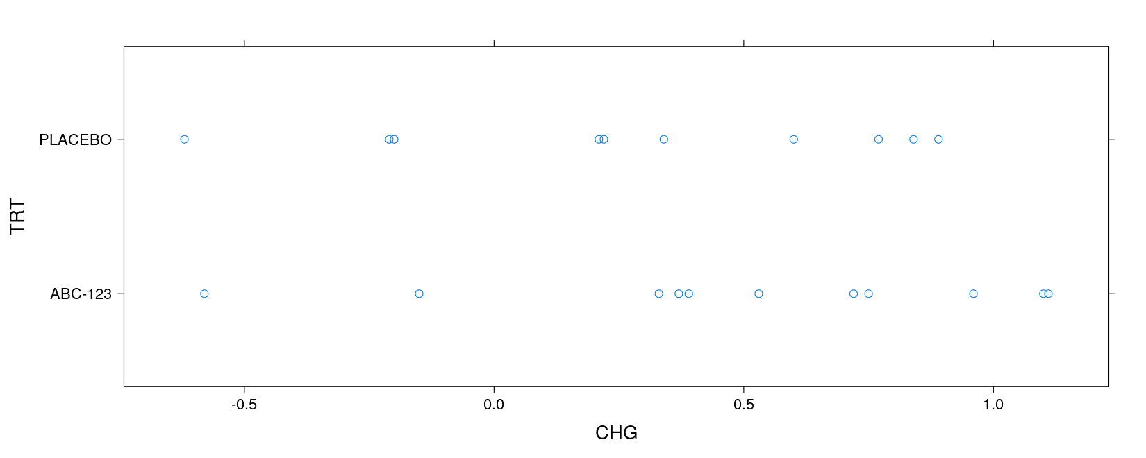
The formula interface for linear models
lm()is an important function that deserves detailed discussionA linear model is any model that can be expressed in the form
y = Xβ + εVery flexible model incorporating ANOVA and linear regression (including some spline models)
The role of the formula in
lm(formula, data)is to specify y and X in terms of variables indataBasic form:
y ~ model, whereyis the name of the response variablemodelconsists of a series of terms separated by+Each term is usually a predictor by itself (main effect), or an interaction
Terms can be functions of variables, possibly a matrix (e.g.,
log(x),poly(x, 2))Interactions are defined using a
:(e.g.,a:b)The intercept term is represented by
1In R, each term is a symbolic representation, not the actual columns of X
Each term gets expanded into one or more columns in X (using
model.matrix())Some shortcuts:
y ~ a * bis equivalent toy ~ a + b + a:by ~ a * b * cis equivalent toy ~ a + b + c + a:b + b:c + c:a + a:b:cy ~ (a + b + c)^2is equivalent toy ~ a + b + c + a:b + b:c + c:a
y ~ a * b * c - a:b:cis also equivalent toy ~ a + b + c + a:b + b:c + c:ay ~ xis equivalent toy ~ 1 + x(intercept term is implied)y ~ x - 1andy ~ 0 + xexplicitly removes the intercept termSee
help(formula)for more details
Obtaining the model matrix
R converts each model specification into a model matrix X
Numeric predictors are retained as they are
Categorical predictors are converted using a full rank re-parameterization (which can be customized)
By default, the first column of the dummy variable matrix is omitted
Remaining coefficients represent “effect compared to first (omitted) level”
Example: Simple Linear Regression
   (Intercept) age
1            1  37
2            1  65
3            1  32
4            1  23
5            1  44
6            1  49
7            1  35
8            1  50
9            1  49
10           1  60
11           1  39
12           1  67
13           1  70
14           1  55
15           1  65
16           1  45
17           1  36
18           1  46
19           1  44
20           1  77
21           1  45
22           1  59
23           1  49
24           1  33
25           1  33
26           1  44
27           1  64
28           1  56
29           1  73
30           1  46
31           1  44
32           1  53
33           1  45
34           1  65
35           1  43
36           1  39
37           1  50
38           1  30
39           1  33
40           1  65
41           1  57
42           1  56
43           1  67
44           1  46
45           1  72
46           1  29
47           1  65
48           1  46
49           1  60
50           1  28
51           1  44
52           1  66
53           1  46
54           1  75
55           1  46
56           1  55
57           1  57
58           1  63
59           1  61
60           1  49
attr(,"assign")
[1] 0 1
Example: Additive effect of group
   (Intercept) age genderFemale
1            1  37            0
2            1  65            1
3            1  32            0
4            1  23            1
5            1  44            0
6            1  49            1
7            1  35            0
8            1  50            1
9            1  49            0
10           1  60            1
11           1  39            0
12           1  67            1
13           1  70            0
14           1  55            0
15           1  65            0
16           1  45            0
17           1  36            0
18           1  46            0
19           1  44            1
20           1  77            1
21           1  45            0
22           1  59            0
23           1  49            1
24           1  33            0
25           1  33            0
26           1  44            1
27           1  64            0
28           1  56            0
29           1  73            0
30           1  46            0
31           1  44            0
32           1  53            1
33           1  45            0
34           1  65            0
35           1  43            1
36           1  39            0
37           1  50            0
38           1  30            1
39           1  33            1
40           1  65            0
41           1  57            1
42           1  56            0
43           1  67            0
44           1  46            1
45           1  72            1
46           1  29            0
47           1  65            1
48           1  46            0
49           1  60            0
50           1  28            0
51           1  44            0
52           1  66            1
53           1  46            0
54           1  75            0
55           1  46            0
56           1  55            1
57           1  57            1
58           1  63            0
59           1  61            0
attr(,"assign")
[1] 0 1 2
attr(,"contrasts")
attr(,"contrasts")$gender
[1] "contr.treatment"
Example: Interaction
   (Intercept) age genderFemale age:genderFemale
1            1  37            0                0
2            1  65            1               65
3            1  32            0                0
4            1  23            1               23
5            1  44            0                0
6            1  49            1               49
7            1  35            0                0
8            1  50            1               50
9            1  49            0                0
10           1  60            1               60
11           1  39            0                0
12           1  67            1               67
13           1  70            0                0
14           1  55            0                0
15           1  65            0                0
16           1  45            0                0
17           1  36            0                0
18           1  46            0                0
19           1  44            1               44
20           1  77            1               77
21           1  45            0                0
22           1  59            0                0
23           1  49            1               49
24           1  33            0                0
25           1  33            0                0
26           1  44            1               44
27           1  64            0                0
28           1  56            0                0
29           1  73            0                0
30           1  46            0                0
31           1  44            0                0
32           1  53            1               53
33           1  45            0                0
34           1  65            0                0
35           1  43            1               43
36           1  39            0                0
37           1  50            0                0
38           1  30            1               30
39           1  33            1               33
40           1  65            0                0
41           1  57            1               57
42           1  56            0                0
43           1  67            0                0
44           1  46            1               46
45           1  72            1               72
46           1  29            0                0
47           1  65            1               65
48           1  46            0                0
49           1  60            0                0
50           1  28            0                0
51           1  44            0                0
52           1  66            1               66
53           1  46            0                0
54           1  75            0                0
55           1  46            0                0
56           1  55            1               55
57           1  57            1               57
58           1  63            0                0
59           1  61            0                0
attr(,"assign")
[1] 0 1 2 3
attr(,"contrasts")
attr(,"contrasts")$gender
[1] "contr.treatment"
Example: All second-order interactions
(Intercept) age genderFemale raceBlack raceOther age:genderFemale age:raceBlack age:raceOther
1 1 37 0 0 1 0 0 37
2 1 65 1 0 0 65 0 0
3 1 32 0 1 0 0 32 0
4 1 23 1 0 0 23 0 0
5 1 44 0 0 1 0 0 44
6 1 49 1 0 0 49 0 0
7 1 35 0 0 1 0 0 35
8 1 50 1 0 0 50 0 0
9 1 49 0 1 0 0 49 0
10 1 60 1 0 0 60 0 0
11 1 39 0 0 1 0 0 39
12 1 67 1 0 0 67 0 0
13 1 70 0 0 0 0 0 0
14 1 55 0 1 0 0 55 0
15 1 65 0 0 0 0 0 0
16 1 45 0 0 0 0 0 0
17 1 36 0 0 0 0 0 0
18 1 46 0 1 0 0 46 0
19 1 44 1 0 0 44 0 0
20 1 77 1 1 0 77 77 0
21 1 45 0 0 0 0 0 0
22 1 59 0 0 0 0 0 0
23 1 49 1 0 0 49 0 0
24 1 33 0 1 0 0 33 0
25 1 33 0 1 0 0 33 0
26 1 44 1 0 0 44 0 0
27 1 64 0 0 0 0 0 0
28 1 56 0 0 1 0 0 56
29 1 73 0 1 0 0 73 0
30 1 46 0 0 0 0 0 0
31 1 44 0 1 0 0 44 0
32 1 53 1 0 0 53 0 0
33 1 45 0 0 0 0 0 0
34 1 65 0 0 1 0 0 65
35 1 43 1 1 0 43 43 0
36 1 39 0 0 0 0 0 0
37 1 50 0 0 0 0 0 0
38 1 30 1 1 0 30 30 0
39 1 33 1 0 0 33 0 0
40 1 65 0 0 0 0 0 0
41 1 57 1 0 0 57 0 0
42 1 56 0 1 0 0 56 0
43 1 67 0 0 0 0 0 0
44 1 46 1 1 0 46 46 0
45 1 72 1 0 0 72 0 0
46 1 29 0 0 0 0 0 0
47 1 65 1 0 0 65 0 0
48 1 46 0 1 0 0 46 0
49 1 60 0 0 0 0 0 0
50 1 28 0 0 0 0 0 0
51 1 44 0 1 0 0 44 0
52 1 66 1 0 0 66 0 0
53 1 46 0 1 0 0 46 0
54 1 75 0 0 0 0 0 0
55 1 46 0 0 0 0 0 0
56 1 55 1 0 0 55 0 0
57 1 57 1 1 0 57 57 0
58 1 63 0 0 0 0 0 0
59 1 61 0 1 0 0 61 0
genderFemale:raceBlack genderFemale:raceOther
1 0 0
2 0 0
3 0 0
4 0 0
5 0 0
6 0 0
7 0 0
8 0 0
9 0 0
10 0 0
11 0 0
12 0 0
13 0 0
14 0 0
15 0 0
16 0 0
17 0 0
18 0 0
19 0 0
20 1 0
21 0 0
22 0 0
23 0 0
24 0 0
25 0 0
26 0 0
27 0 0
28 0 0
29 0 0
30 0 0
31 0 0
32 0 0
33 0 0
34 0 0
35 1 0
36 0 0
37 0 0
38 1 0
39 0 0
40 0 0
41 0 0
42 0 0
43 0 0
44 1 0
45 0 0
46 0 0
47 0 0
48 0 0
49 0 0
50 0 0
51 0 0
52 0 0
53 0 0
54 0 0
55 0 0
56 0 0
57 1 0
58 0 0
59 0 0
attr(,"assign")
[1] 0 1 2 3 3 4 5 5 6 6
attr(,"contrasts")
attr(,"contrasts")$gender
[1] "contr.treatment"
attr(,"contrasts")$race
[1] "contr.treatment"Fitting a linear model
'data.frame':   93 obs. of  27 variables:
 $ Manufacturer      : Factor w/ 32 levels "Acura","Audi",..: 1 1 2 2 3 4 4 4 4 5 ...
 $ Model             : Factor w/ 93 levels "100","190E","240",..: 49 56 9 1 6 24 54 74 73 35 ...
 $ Type              : Factor w/ 6 levels "Compact","Large",..: 4 3 1 3 3 3 2 2 3 2 ...
 $ Min.Price         : num  12.9 29.2 25.9 30.8 23.7 14.2 19.9 22.6 26.3 33 ...
 $ Price             : num  15.9 33.9 29.1 37.7 30 15.7 20.8 23.7 26.3 34.7 ...
 $ Max.Price         : num  18.8 38.7 32.3 44.6 36.2 17.3 21.7 24.9 26.3 36.3 ...
 $ MPG.city          : int  25 18 20 19 22 22 19 16 19 16 ...
 $ MPG.highway       : int  31 25 26 26 30 31 28 25 27 25 ...
 $ AirBags           : Factor w/ 3 levels "Driver & Passenger",..: 3 1 2 1 2 2 2 2 2 2 ...
 $ DriveTrain        : Factor w/ 3 levels "4WD","Front",..: 2 2 2 2 3 2 2 3 2 2 ...
 $ Cylinders         : Factor w/ 6 levels "3","4","5","6",..: 2 4 4 4 2 2 4 4 4 5 ...
 $ EngineSize        : num  1.8 3.2 2.8 2.8 3.5 2.2 3.8 5.7 3.8 4.9 ...
 $ Horsepower        : int  140 200 172 172 208 110 170 180 170 200 ...
 $ RPM               : int  6300 5500 5500 5500 5700 5200 4800 4000 4800 4100 ...
 $ Rev.per.mile      : int  2890 2335 2280 2535 2545 2565 1570 1320 1690 1510 ...
 $ Man.trans.avail   : Factor w/ 2 levels "No","Yes": 2 2 2 2 2 1 1 1 1 1 ...
 $ Fuel.tank.capacity: num  13.2 18 16.9 21.1 21.1 16.4 18 23 18.8 18 ...
 $ Passengers        : int  5 5 5 6 4 6 6 6 5 6 ...
 $ Length            : int  177 195 180 193 186 189 200 216 198 206 ...
 $ Wheelbase         : int  102 115 102 106 109 105 111 116 108 114 ...
 $ Width             : int  68 71 67 70 69 69 74 78 73 73 ...
 $ Turn.circle       : int  37 38 37 37 39 41 42 45 41 43 ...
 $ Rear.seat.room    : num  26.5 30 28 31 27 28 30.5 30.5 26.5 35 ...
 $ Luggage.room      : int  11 15 14 17 13 16 17 21 14 18 ...
 $ Weight            : int  2705 3560 3375 3405 3640 2880 3470 4105 3495 3620 ...
 $ Origin            : Factor w/ 2 levels "USA","non-USA": 2 2 2 2 2 1 1 1 1 1 ...
 $ Make              : Factor w/ 93 levels "Acura Integra",..: 1 2 4 3 5 6 7 9 8 10 ...
Linear models are fit using
lm()The result is usually stored in a variable for further processing
The return value of lm()
lm()returns a listThe meaning of most components are obvious, but see
help(lm)for details
List of 13
 $ coefficients : Named num [1:12] 41.3291 -0.0062 10.277 -4.0899 1.1735 ...
 $ residuals    : Named num [1:93] 0.788 0.733 0.461 0.237 4.858 ...
 $ effects      : Named num [1:93] -215.69 45.45 4.9 1.25 1.28 ...
 $ rank         : int 12
 $ fitted.values: Named num [1:93] 24.2 17.3 19.5 18.8 17.1 ...
 $ assign       : int [1:12] 0 1 2 3 3 4 5 5 6 6 ...
 $ qr           :List of 5
  ..$ qr   : num [1:93, 1:12] -9.644 0.104 0.104 0.104 0.104 ...
  ..$ qraux: num [1:12] 1.1 1.09 1.12 1.11 1.04 ...
  ..$ pivot: int [1:12] 1 2 3 4 5 6 7 8 9 10 ...
  ..$ tol  : num 1e-07
  ..$ rank : int 12
 $ df.residual  : int 81
 $ contrasts    :List of 2
  ..$ Man.trans.avail: chr "contr.treatment"
  ..$ AirBags        : chr "contr.treatment"
 $ xlevels      :List of 2
  ..$ Man.trans.avail: chr [1:2] "No" "Yes"
  ..$ AirBags        : chr [1:3] "Driver & Passenger" "Driver only" "None"
 $ call         : language lm(formula = MPG.city ~ Weight * Man.trans.avail * AirBags, data = Cars93)
 $ terms        :Classes 'terms', 'formula'  language MPG.city ~ Weight * Man.trans.avail * AirBags
 $ model        :'data.frame':  93 obs. of  4 variables:
  ..$ MPG.city       : int [1:93] 25 18 20 19 22 22 19 16 19 16 ...
  ..$ Weight         : int [1:93] 2705 3560 3375 3405 3640 2880 3470 4105 3495 3620 ...
  ..$ Man.trans.avail: Factor w/ 2 levels "No","Yes": 2 2 2 2 2 1 1 1 1 1 ...
  ..$ AirBags        : Factor w/ 3 levels "Driver & Passenger",..: 3 1 2 1 2 2 2 2 2 2 ...
Using the fitted model: summary()
- Performs a t-test for each column of X (does not always make sense)
Call:
lm(formula = MPG.city ~ Weight * Man.trans.avail * AirBags, data = Cars93)

Residuals:
    Min      1Q  Median      3Q     Max
-6.8822 -1.3541 -0.0079  0.8039 13.1871

Coefficients:
                                               Estimate Std. Error t value Pr(>|t|)
(Intercept)                                  41.3291301 13.6733416   3.023  0.00335 **
Weight                                       -0.0062036  0.0037873  -1.638  0.10530
Man.trans.availYes                           10.2770284 20.9825645   0.490  0.62561
AirBagsDriver only                           -4.0898583 15.4854474  -0.264  0.79237
AirBagsNone                                   1.1735115 17.1752446   0.068  0.94569
Weight:Man.trans.availYes                    -0.0034421  0.0061659  -0.558  0.57821
Weight:AirBagsDriver only                     0.0010294  0.0043071   0.239  0.81172
Weight:AirBagsNone                           -0.0003477  0.0047409  -0.073  0.94171
Man.trans.availYes:AirBagsDriver only         2.5575320 22.5411909   0.113  0.90995
Man.trans.availYes:AirBagsNone                1.8911293 23.6413834   0.080  0.93644
Weight:Man.trans.availYes:AirBagsDriver only -0.0004309  0.0066246  -0.065  0.94830
Weight:Man.trans.availYes:AirBagsNone        -0.0012667  0.0069125  -0.183  0.85506
---
Signif. codes:  0 '***' 0.001 '**' 0.01 '*' 0.05 '.' 0.1 ' ' 1

Residual standard error: 3.005 on 81 degrees of freedom
Multiple R-squared:  0.7483,    Adjusted R-squared:  0.7141
F-statistic: 21.89 on 11 and 81 DF,  p-value: < 2.2e-16
Using the fitted model: anova()
- Performs sequential F-tests (using the order in which terms were added)
Analysis of Variance Table

Response: MPG.city
                               Df  Sum Sq Mean Sq  F value  Pr(>F)
Weight                          1 2065.52 2065.52 228.7639 < 2e-16 ***
Man.trans.avail                 1   24.01   24.01   2.6592 0.10684
AirBags                         2    3.20    1.60   0.1772 0.83794
Weight:Man.trans.avail          1   55.14   55.14   6.1064 0.01557 *
Weight:AirBags                  2    0.63    0.32   0.0350 0.96565
Man.trans.avail:AirBags         2   25.20   12.60   1.3954 0.25362
Weight:Man.trans.avail:AirBags  2    0.52    0.26   0.0290 0.97143
Residuals                      81  731.35    9.03
---
Signif. codes: 0 '***' 0.001 '**' 0.01 '*' 0.05 '.' 0.1 ' ' 1- Can also be used to compare two arbitrary (nested) models
Analysis of Variance Table

Model 1: MPG.city ~ Weight
Model 2: MPG.city ~ Weight * Man.trans.avail * AirBags
  Res.Df    RSS Df Sum of Sq      F Pr(>F)
1     91 840.05
2     81 731.35 10     108.7 1.2039 0.3011
Using the fitted model: coefficients()
                                 (Intercept)                                       Weight
                               41.3291300743                                -0.0062036131
                          Man.trans.availYes                           AirBagsDriver only
                               10.2770283603                                -4.0898583382
                                 AirBagsNone                    Weight:Man.trans.availYes
                                1.1735114521                                -0.0034420884
                   Weight:AirBagsDriver only                           Weight:AirBagsNone
                                0.0010293517                                -0.0003477101
       Man.trans.availYes:AirBagsDriver only               Man.trans.availYes:AirBagsNone
                                2.5575320500                                 1.8911292706
Weight:Man.trans.availYes:AirBagsDriver only        Weight:Man.trans.availYes:AirBagsNone
                               -0.0004308614                                -0.0012666999
Using the fitted model: Residuals and fitted values
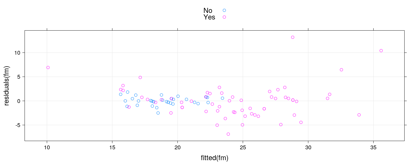
Summary: common interface
Most modeling functions in R support the formula interface
Most also support some common methods:
coef()to obtain coefficientsfitted()to get fitted valuesresiduals()to get residualspredict()to get predicted values for new predictor values
Contingency tables
Contingency tables can be created using
table()orxtabs()Essentially same, but
xtabs()uses a formula-data interface
       trt
race    Active Placebo
  White     18      18
  Black     10       8
Other 3 3 trt
gender Active Placebo
Male 22 16
Female 9 12- Fisher’s exact test is performed using
fisher.test()
tt.gender <- xtabs(~ gender + trt, data = demog)
tt.race <- xtabs(~ race + trt, data = demog)
fisher.test(tt.gender)
    Fisher's Exact Test for Count Data

data:  tt.gender
p-value = 0.2911
alternative hypothesis: true odds ratio is not equal to 1
95 percent confidence interval:
 0.5486984 6.2107193
sample estimates:
odds ratio
  1.814327
    Fisher's Exact Test for Count Data

data:  tt.race
p-value = 0.927
alternative hypothesis: two.sided- The χ2-test is performed using
chisq.test()
    Pearson's Chi-squared test with Yates' continuity correction

data:  tt.gender
X-squared = 0.69763, df = 1, p-value = 0.4036
    Pearson's Chi-squared test

data:  tt.gender
X-squared = 1.2266, df = 1, p-value = 0.2681Warning in chisq.test(tt.race): Chi-squared approximation may be incorrect
    Pearson's Chi-squared test

data:  tt.race
X-squared = 0.15573, df = 2, p-value = 0.9251
Survival models
- Use survival data in the file data/death.txt
death <- read.table("data/death.txt", header = TRUE, na.strings = ".", stringsAsFactors = FALSE)
death <- within(death,
{
    trt <- factor(trt, levels = c("A", "B", "C"),
                  labels = c("Placebo", "Old Drug", "New Drug"))
    monthstodeath <- daystodeath / (365.25 / 12) # survival time in months
})
str(death)
'data.frame': 200 obs. of 4 variables:
$ trt : Factor w/ 3 levels "Placebo","Old Drug",..: 1 1 3 3 2 2 2 2 3 3 ...
$ daystodeath : int 52 825 693 981 279 826 531 15 1057 793 ...
$ deathcensor : int 1 0 0 0 1 0 0 0 0 0 ...
$ monthstodeath: num 1.71 27.1 22.77 32.23 9.17 ...deathcensoris 1 if the patient died, and 0 if the survival time was censoredKaplan-Meier survival curves are fit using
survfit()in the survival packageThe model formula needs a survival object created using
Surv()A survival objects needs the survival times and the censoring indicator
  [1]  1.70841889  27.10472279+ 22.76796715+ 32.22997947+  9.16632444  27.13757700+ 17.44558522+  0.49281314+
  [9] 34.72689938+ 26.05338809+ 34.43121150+ 30.39014374+ 15.44147844+  8.24640657  27.26899384+ 21.94661191
 [17] 11.49897331+ 24.50924025+  4.00821355  27.10472279+  5.35523614  24.14784394+ 22.96509240+ 25.33059548
 [25] 29.20739220+ 30.62012320+ 25.39630390  25.19917864+  5.09240246+ 23.26078029+ 17.97125257+ 15.17864476
 [33]  3.74537988  23.12936345+ 34.29979466+ 23.06365503  26.80903491+  3.28542094  31.31006160+ 20.76386037+
 [41] 31.50718686+ 22.17659138+ 31.54004107   1.67556468+  1.08418891  21.19096509+  1.83983573  32.19712526
 [49]  4.92813142+ 20.96098563+ 29.73305955+ 11.20328542  22.53798768+ 20.96098563+ 28.64887064  44.25462012+
 [57] 21.65092402+  4.36960986  11.82751540+ 29.79876797   2.29979466+ 19.44969199+  3.67967146+ 28.97741273
 [65] 33.08418891+ 19.51540041+  0.22997947+ 11.86036961+ 31.67145791+ 19.12114990+ 33.64271047  17.74127310
 [73] 31.60574949+  9.26488706+ 28.68172485+ 42.51334702+ 31.57289528+ 17.11704312+  8.80492813  21.58521561+
 [81] 32.85420945+  0.29568789  22.27515400+ 32.49281314  29.89733060+ 36.36960986+ 35.18685832  31.90143737+
 [89]  2.92402464+ 36.50102669+ 23.03080082+ 11.95893224  14.52156057   3.02258727  35.44969199+  3.05544148+
 [97] 17.47843943  34.89117043+ 29.66735113+ 26.02053388+  4.46817248+  5.05954825+ 27.76180698+  1.70841889+
[105] 27.56468172+ 35.35112936+ 27.40041068  19.35112936+ 26.77618070+ 34.06981520+ 27.33470226+ 36.79671458+
[113] 26.38193018+  0.52566735  20.69815195+ 17.93839836+  0.91991786  32.98562628+ 33.51129363+  2.46406571+
[121] 42.67761807+  2.59548255+  5.58521561+ 31.04722793+ 34.69404517+ 31.11293634+ 33.34702259+  6.24229979
[129] 33.70841889+  4.20533881  30.88295688+ 41.72484600+ 33.57700205  30.06160164+ 14.02874743   5.81519507
[137]  4.17248460+ 24.47638604  27.40041068+ 24.70636550+ 39.72073922+  5.05954825+ 23.75359343+ 40.87063655+
[145]  0.16427105+ 27.36755647+ 23.16221766+  1.60985626+ 31.34291581+  1.97125257  23.16221766+ 17.34702259+
[153] 31.27720739+ 25.49486653+ 22.34086242+  2.89117043+  0.75564682+ 25.49486653+ 21.91375770+  5.09240246+
[161] 31.08008214+ 24.70636550+ 35.35112936+ 12.48459959  31.04722793+ 23.72073922+ 20.69815195+  2.00410678
[169] 30.58726899+  0.06570842+ 19.15400411+  9.26488706   3.38398357  34.03696099+ 19.67967146+  0.55852156+
[177] 29.89733060+ 24.96919918+ 18.49691992+ 11.40041068  29.79876797+ 29.43737166+ 17.87268994+ 13.27310062
[185]  0.26283368  29.40451745+ 17.24845996+ 24.31211499+  0.36139630+ 14.65297741  17.14989733+  8.34496920+
[193] 28.51745380+ 25.42915811+ 16.42710472+  0.88706366+ 27.66324435+  8.80492813  16.59137577+ 16.59137577
Kaplan-Meier survival estimate by treatment subgroup
Call: survfit(formula = Surv(monthstodeath, deathcensor) ~ trt, data = death)

              n events median 0.95LCL 0.95UCL
trt=Placebo  68     26   32.2    28.6      NA
trt=Old Drug 64     18     NA    33.6      NA
trt=New Drug 68 7 NA NA NA- Estimated survival probability upto specified times are given by the
summary()method
Call: survfit(formula = Surv(monthstodeath, deathcensor) ~ trt, data = death)

                trt=Placebo
 time n.risk n.event survival std.err lower 95% CI upper 95% CI
    0     68       0    1.000  0.0000        1.000        1.000
    3     61       4    0.940  0.0291        0.885        0.999
    6     53       6    0.845  0.0450        0.762        0.938
   12     48       5    0.766  0.0530        0.668        0.877
   24     27       6    0.662  0.0608        0.553        0.793
   36      2       5    0.395  0.1137        0.225        0.695

                trt=Old Drug
 time n.risk n.event survival std.err lower 95% CI upper 95% CI
    0     64       0    1.000  0.0000        1.000        1.000
    3     55       4    0.935  0.0316        0.875        0.999
    6     52       2    0.900  0.0387        0.828        0.979
   12     45       4    0.829  0.0493        0.738        0.932
   24     29       4    0.751  0.0583        0.645        0.874

                trt=New Drug
 time n.risk n.event survival std.err lower 95% CI upper 95% CI
    0     68       0    1.000  0.0000        1.000        1.000
    3     59       1    0.985  0.0153        0.955        1.000
    6     51       1    0.968  0.0225        0.924        1.000
   12     49       0    0.968  0.0225        0.924        1.000
   24     35       1    0.948  0.0295        0.892        1.000
36 7 4 0.713 0.1129 0.523 0.973- Survival curves can be plotted using the
summary()method
plot(sm, mark.time = TRUE, col = 1:3,
     xlab = "Months from Randomization",
     main = "Kaplan-Meier Survival Estimates for Death")
legend("bottomleft", names(sm$strata), inset = 0.01, lty = 1, col = 1:3)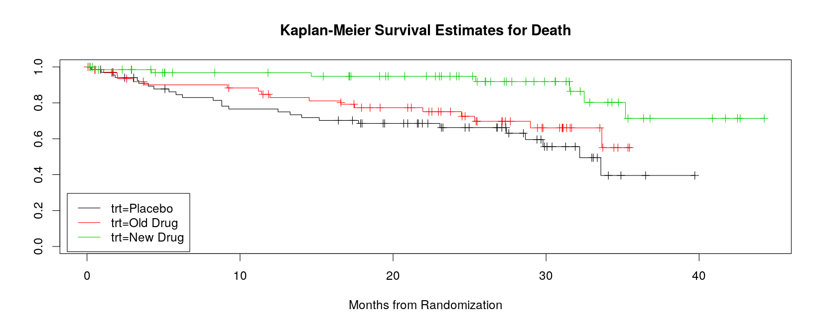
Test for differences in survival by treatment subgroup
- Equality of survival curves can be tested using
survdiff()
Call:
survdiff(formula = Surv(monthstodeath, deathcensor) ~ trt, data = death,
    rho = 0)

              N Observed Expected (O-E)^2/E (O-E)^2/V
trt=Placebo  68       26     16.2     5.885     8.697
trt=Old Drug 64       18     15.9     0.288     0.421
trt=New Drug 68        7     18.9     7.502    12.166

Chisq= 13.9 on 2 degrees of freedom, p= 9e-04 Call:
survdiff(formula = Surv(monthstodeath, deathcensor) ~ trt, data = death,
rho = 1)
N Observed Expected (O-E)^2/E (O-E)^2/V
trt=Placebo 68 22.43 14.0 5.145 8.803
trt=Old Drug 64 15.40 13.6 0.245 0.413
trt=New Drug 68 5.45 15.7 6.731 12.512
Chisq= 14.3 on 2 degrees of freedom, p= 8e-04 Exercises
- Perform a one-sample t-test to answer the following question:
In a number of previous Phase I and II studies of male, non-insulin-dependent diabetic (NIDDM) patients, the mean body mass index (BMI) was found to be 28.4. An investigator has 17 male NIDDM patients enrolled in a new study and wants to know if the BMI from this sample is consistent with previous findings. BMI is computed as the ratio of weight in kilograms to the square of the height in meters. What conclusion can the investigator make based on the following height and weight data from his 17 patients?
- Data is available in the file sasdata/onesample.sas7bdat
- Perform an appropriate ANOVA test to answer the following question:
A new synthetic erythropoietin-type hormone, Rebligen, which is used to treat chemotherapy-induced anemia in cancer patients, was tested in a study of 48 adult cancer patients undergoing chemotherapeutic treatment. Half the patients received low-dose administration of Rebligen via intramuscular injection three times at 2-day intervals, and half the patients received a placebo in a similar fashion. Patients were stratified according to their type of cancer: cervical, prostate, or colorectal. Changes in hemoglobin (in mg/dl) from pre-first injection to one week after last injection were obtained for analysis. Does Rebligen have any effect on the hemoglobin (Hgb) levels?
- data is available in the file sasdata/anova.sas7bdat
- Create contingency tables and perform tests of independence to answer the following question:
A study was conducted to monitor the incidence of gastro-intestinal (GI) adverse drug reactions of a new antibiotic used in lower respiratory tract infections (LRTI). Two parallel groups were included in the study. One group consisted of 66 LRTI patients randomized to receive the new treatment, and a reference group of 52 LRTI patients were randomized to receive erythromycin. There were 22 patients in the test group and 28 patients in the control (erythromycin) group who reported one or more GI complaints during 7 days of treatment. Is there evidence of a difference in GI side effect rates between the two groups?
First, construct the contingency table by hand and perform the test
Also read in the dataset sasdata/chisqr.sas7bdat and construct the contingency table from it. Note that the data is already summarized; read
help(xtabs)and use an appropriate variable in the left hand side of the formula to construct the contingency table