Writing R Functions
Functions in R
A tutorial on R would be incomplete without a discussion of functions
R provides most of its functionality through functions
However, it by design does not try to provide functions to satisfy all needs
R users are expected to write their own functions to suit their requirements
Functions are “first class” objects in R
From a language perspective, functions are like any other type of object
They can be bound to variables, and put inside lists
They can be passed as arguments to other functions
In fact, this is very common, and we will see many such examples
Creating functions
- Functions are created using the following structure:
Here
argsis a comma-separated list of variables (arguments) that are available to the functionThe instructions are R code that is executed whenever the function is run
Every function must return a value
The return value can be explicit using
return(), otherwise it is the last evaluated expressionSee
help("function")(note that the quotes are required)Without going into technical detail, we will learn through examples
Functions can be very simple. For example:
We are interested in the p-value for many of the tests we do
However, R doesn’t have a function that provides just the p-value
To extract the p-value from a test, we need to know its internal structure
We can define a function to extract p-values as follows:
- Let’s read in the
demogdata again:
demog <- read.table("data/demog.txt", header = TRUE, na.strings = ".", stringsAsFactors = FALSE)
demog <- within(demog,
{
    trt = factor(trt, levels = c(1, 0), labels = c("Active", "Placebo"))
    gender = factor(gender, levels = c(1, 2), labels = c("Male", "Female"))
    race = factor(race, levels = c(1, 2, 3), labels = c("White", "Black", "Other"))
})
str(demog)
'data.frame': 60 obs. of 5 variables:
$ subjid: int 101 102 103 104 105 106 201 202 203 204 ...
$ trt : Factor w/ 2 levels "Active","Placebo": 2 1 1 2 1 2 1 2 1 2 ...
$ gender: Factor w/ 2 levels "Male","Female": 1 2 1 2 1 2 1 2 1 2 ...
$ race : Factor w/ 3 levels "White","Black",..: 3 1 2 1 3 1 3 1 2 1 ...
$ age : int 37 65 32 23 44 49 35 50 49 60 ...- And extract the p-values for various tests
[1] 0.7155171[1] 0.7155208[1] 0.2910557[1] 0.4035804NULLp-value for linear models
Our function doesn’t work for
lm()fitsThis is because
"lm"objects do not store a p-value as the$p.valuecomponentIn fact, a linear model can lead to many tests, and it is not clear which p-value should be reported
It is conventional to report the p-value of the test comparing full model with intercept-only model
This is shown as the last result in
summary()
Call:
lm(formula = age ~ race, data = demog)

Residuals:
    Min      1Q  Median      3Q     Max
-29.722  -7.722  -2.389  10.528  28.611

Coefficients:
            Estimate Std. Error t value Pr(>|t|)
(Intercept)   52.722      2.185  24.133   <2e-16 ***
raceBlack     -4.333      3.784  -1.145    0.257
raceOther     -6.722      5.780  -1.163    0.250
---
Signif. codes:  0 '***' 0.001 '**' 0.01 '*' 0.05 '.' 0.1 ' ' 1

Residual standard error: 13.11 on 57 degrees of freedom
Multiple R-squared:  0.03695,   Adjusted R-squared:  0.003158
F-statistic: 1.093 on 2 and 57 DF, p-value: 0.342- However, it can be quite frustrating to figure out where this p-value is calculated
List of 11
 $ call         : language lm(formula = age ~ race, data = demog)
 $ terms        :Classes 'terms', 'formula'  language age ~ race
  .. ..- attr(*, "variables")= language list(age, race)
  .. ..- attr(*, "factors")= int [1:2, 1] 0 1
  .. .. ..- attr(*, "dimnames")=List of 2
  .. .. .. ..$ : chr [1:2] "age" "race"
  .. .. .. ..$ : chr "race"
  .. ..- attr(*, "term.labels")= chr "race"
  .. ..- attr(*, "order")= int 1
  .. ..- attr(*, "intercept")= int 1
  .. ..- attr(*, "response")= int 1
  .. ..- attr(*, ".Environment")=<environment: R_GlobalEnv>
  .. ..- attr(*, "predvars")= language list(age, race)
  .. ..- attr(*, "dataClasses")= Named chr [1:2] "numeric" "factor"
  .. .. ..- attr(*, "names")= chr [1:2] "age" "race"
 $ residuals    : Named num [1:60] -9 12.3 -16.4 -29.7 -2 ...
  ..- attr(*, "names")= chr [1:60] "1" "2" "3" "4" ...
 $ coefficients : num [1:3, 1:4] 52.72 -4.33 -6.72 2.18 3.78 ...
  ..- attr(*, "dimnames")=List of 2
  .. ..$ : chr [1:3] "(Intercept)" "raceBlack" "raceOther"
  .. ..$ : chr [1:4] "Estimate" "Std. Error" "t value" "Pr(>|t|)"
 $ aliased      : Named logi [1:3] FALSE FALSE FALSE
  ..- attr(*, "names")= chr [1:3] "(Intercept)" "raceBlack" "raceOther"
 $ sigma        : num 13.1
 $ df           : int [1:3] 3 57 3
 $ r.squared    : num 0.0369
 $ adj.r.squared: num 0.00316
 $ fstatistic   : Named num [1:3] 1.09 2 57
  ..- attr(*, "names")= chr [1:3] "value" "numdf" "dendf"
 $ cov.unscaled : num [1:3, 1:3] 0.0278 -0.0278 -0.0278 -0.0278 0.0833 ...
  ..- attr(*, "dimnames")=List of 2
  .. ..$ : chr [1:3] "(Intercept)" "raceBlack" "raceOther"
  .. ..$ : chr [1:3] "(Intercept)" "raceBlack" "raceOther"
 - attr(*, "class")= chr "summary.lm"
It turns out that the calculation is done in the
print()method for"summary.lm"objectsThe following shows the relevant part of the method
    ...
    if (!is.null(x$fstatistic)) {
        cat("Multiple R-squared: ", formatC(x$r.squared, digits = digits))
        cat(",\tAdjusted R-squared: ", formatC(x$adj.r.squared,
            digits = digits), "\nF-statistic:", formatC(x$fstatistic[1L],
            digits = digits), "on", x$fstatistic[2L], "and",
            x$fstatistic[3L], "DF,  p-value:", format.pval(pf(x$fstatistic[1L],
                x$fstatistic[2L], x$fstatistic[3L], lower.tail = FALSE),
                digits = digits))
        cat("\n")
    }
   ...
How does this help us?
A more flexible design for our
pvalue()function:Make the function generic
Write specific methods for
"htest"and"lm"objectsOther types of objects can be supported in future by adding suitable methods
Generic function with methods
pvalue <- function(x) UseMethod("pvalue")
pvalue.htest <- function(x) x$p.value
pvalue.lm <- function(x)
{
    f <- summary(x)$fstatistic
    if (is.null(f)) stop("p-value not defined") # can happen if model is intercept-only
    pf(f[1], f[2], f[3], lower.tail = FALSE)    # pf gives distribution function of F
}[1] 0.7155171[1] 0.7155208[1] 0.2910557[1] 0.4035804 value
0.3419768 Inspecting functions
All R functions are defined in essentially the same manner
Just like other variables, functions can also be printed
Typing the name of a funtion will usually display its definition
Some functions call C / Fortran code, which will show up as
.Primitive(),.Internal(),.Call(), etc.
function (x, ...) .Primitive("rep")function (x, decreasing = FALSE, ...)
{
if (!is.logical(decreasing) || length(decreasing) != 1L)
stop("'decreasing' must be a length-1 logical vector.\nDid you intend to set 'partial'?")
UseMethod("sort")
}
<bytecode: 0x55ffede5fce0>
<environment: namespace:base>function (x, decreasing = FALSE, na.last = NA, ...)
{
if (is.object(x))
x[order(x, na.last = na.last, decreasing = decreasing)]
else sort.int(x, na.last = na.last, decreasing = decreasing,
...)
}
<bytecode: 0x55ffee708208>
<environment: namespace:base>function (..., na.last = TRUE, decreasing = FALSE, method = c("auto",
"shell", "radix"))
{
z <- list(...)
decreasing <- as.logical(decreasing)
if (length(z) == 1L && is.numeric(x <- z[[1L]]) && !is.object(x) &&
length(x) > 0) {
if (.Internal(sorted_fpass(x, decreasing, na.last)))
return(seq_along(x))
}
method <- match.arg(method)
if (any(vapply(z, is.object, logical(1L)))) {
z <- lapply(z, function(x) if (is.object(x))
as.vector(xtfrm(x))
else x)
return(do.call("order", c(z, list(na.last = na.last,
decreasing = decreasing, method = method))))
}
if (method == "auto") {
useRadix <- all(vapply(z, function(x) {
(is.numeric(x) || is.factor(x) || is.logical(x)) &&
is.integer(length(x))
}, logical(1L)))
method <- if (useRadix)
"radix"
else "shell"
}
if (method != "radix" && !is.na(na.last)) {
return(.Internal(order(na.last, decreasing, ...)))
}
if (method == "radix") {
decreasing <- rep_len(as.logical(decreasing), length(z))
return(.Internal(radixsort(na.last, decreasing, FALSE,
TRUE, ...)))
}
if (any(diff((l.z <- lengths(z)) != 0L)))
stop("argument lengths differ")
na <- vapply(z, is.na, rep.int(NA, l.z[1L]))
ok <- if (is.matrix(na))
rowSums(na) == 0L
else !any(na)
if (all(!ok))
return(integer())
z[[1L]][!ok] <- NA
ans <- do.call("order", c(z, list(decreasing = decreasing)))
ans[ok[ans]]
}
<bytecode: 0x55ffed412388>
<environment: namespace:base>Another example: linear regression
- Recall our simulated height-weight example
htwt <- data.frame(height = rnorm(200, mean = 172, sd = 10),   # height in cm
                   bmi = rnorm(200, mean = 22, sd = 2.2))      # bmi (independent of height)
htwt <- transform(htwt, weight = bmi * (height / 100)^2) # weight in kg- Suppose we further switch the height and weight of the first observation
'data.frame':   200 obs. of  3 variables:
 $ height: num  56 166 167 160 172 ...
 $ bmi   : num  22.4 20.5 21.3 22.1 18.3 ...
 $ weight: num  158.1 56.3 59.7 56.8 53.8 ...
Call:
lm(formula = weight ~ height, data = htwt)

Coefficients:
(Intercept)       height
57.21366 0.04832 - Recall that we can also obtain the coefficients by explicitly solving the regression equations
with(htwt,
{
    y <- weight
    X <- cbind(Int = 1, HT = height)
    beta <- solve(crossprod(X), crossprod(X, y)) # better than t(X) %*% X etc.
    beta
})
[,1]
Int 57.21366290
HT 0.04832182Yet another conceptually equivalent method is to minimize the sum of squared errors
R has several general-purpose optimizers, typically used through
optim()At a minimum,
optim()requires a function to be optimized and a starting estimateHere, our “sum-of-squares” function takes a parameter of length-2
SSE <- function(beta)
{
    with(htwt,
    {
        sum((weight - beta[1] - beta[2] * height)^2)
    })
}
(opt.sse <- stats::optim(c(0, 0), SSE))
$par
[1] 57.17301085 0.04852863
$value
[1] 25122.54
$counts
function gradient
121 NA
$convergence
[1] 0
$message
NULL- The benefit of this approach is that we can easily change the objective function
SAE <- function(beta)
{
    with(htwt,
    {
        sum(abs(weight - beta[1] - beta[2] * height)) # sum of absolute errors
    })
}
(opt.sae <- optim(c(0, 0), SAE))
$par
[1] -36.4945566 0.5902061
$value
[1] 1193.13
$counts
function gradient
149 NA
$convergence
[1] 0
$message
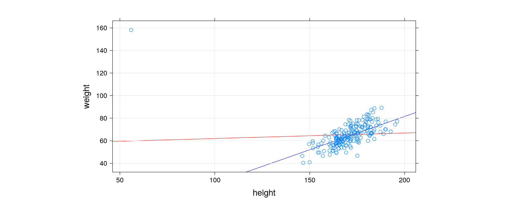
NULLThis is an example of robust regression
library(lattice)
xyplot(weight ~ height, data = htwt, grid = TRUE, aspect = 0.5,
       panel = function(x, y, ...) {
           panel.abline(opt.sse$par, col = "red") # squared errors (influenced by outlier)
           panel.abline(opt.sae$par, col = "blue") # absolute errors
           panel.xyplot(x, y, ...)
       })
The *apply() family of functions
Notice that the second argument of
optim()above is a functionAnother useful class of functions taking other functions as argument: various
apply()type functionsThe most general-purpose among these is
lapply(), which applies a function on all elements of a list
$height
[1] 171.0055

$bmi
[1] 21.98674

$weight
[1] 64.49612- We can also provide a user-defined function here:
mean.and.median <- function(x)
{
    c(mean = mean(x, na.rm = TRUE), median = median(x, na.rm = TRUE))
}
lapply(htwt, mean.and.median)
$height
mean median
170.8390 171.0055
$bmi
mean median
22.07640 21.98674
$weight
mean median
65.46891 64.49612 In fact, the function doesn’t need to have a name
Such functions defined in-place are known as anonymous functions
$height
      SD      IQR
12.45180 13.43753

$bmi
      SD      IQR
2.164412 3.100270

$weight
      SD      IQR
11.25193 12.98609 - This is useful in conjunction with
split()to compute per-group summaries
List of 2
 $ Active : int [1:31] 65 32 44 35 49 39 67 65 36 44 ...
$ Placebo: int [1:29] 37 23 49 50 60 70 55 45 46 77 ...$Active
[1] 51.35484
$Placebo
[1] 50.10345 Active Placebo
51.35484 50.10345 - In fact, this is so common that there is a function called
tapply()to make this easier
  Active  Placebo
51.35484 50.10345
A related function called
apply()is used to apply a function on rows or columns of a matrixWe will use these concepts frequently in the remainder of the workshop