Case Studies
Introduction
In the final session of the workshop, we will consider some more complicated examples that require a non-trivial amount of programming. It is very unlikely that we will be able to cover all the ideas in detail, but you should focus on
first understanding the procedure or algorithm that needs to be implemented,
then understanding how this procedure can be translated into R code.
Importing files
As discussed earlier, the safest way to import data is to use a standard open format such as CSV or other kinds of text files. However, it is often convenient to be able to read data in formats used by SAS.
The most common SAS data format seems to be what is commonly referred to as “SAS7BDAT” (after its standard extension). As far as I can tell, this is an internal binary format with no publicly available official specification, and is not intended for exporting data from SAS to be used by other software such as R. (For such use, one should use SAS to export the data in portable formats such as CSV.)
That said, there is a contributed R package called sas7bdat which is currently able to read in most such files, as long they are not created with the compress=binary option (the default, compress=yes, should be OK).
Another format used by SAS is the SAS XPORT format, which is better documented. The read.xport() function in the foreign package should be able to read most XPORT format files.
For this session, we will use a mix of all three kinds of datasets (txt, sas7bdat, xpt).
ANOVA test and Least Square Means
A new synthetic erythropoietin-type hormone, Rebligen, which is used to treat chemotherapy-induced anemia in cancer patients, was tested in a study of 48 adult cancer patients undergoing chemotherapeutic treatment. Half the patients received low-dose administration of Rebligen via intramuscular injection three times at 2-day intervals; half the patients received a placebo in a similar fashion. Patients were stratified according to their type of cancer: cervical, prostate, or colorectal. For study admission, patients were required to have a baseline hemoglobin less than 10 mg/dl and a decrease in hemoglobin of at least 1 mg/dl following the last chemotherapy. Changes in hemoglobin (in mg/dl) from pre-first injection to one week after last injection (as shown in Table 7.3) were obtained for analysis. Does Rebligen have any effect on the hemoglobin (Hgb) levels?
   PATNO     TRT     TYPE HGBCH
1      1  ACTIVE CERVICAL   1.7
2      3  ACTIVE CERVICAL  -0.2
3      6  ACTIVE CERVICAL   1.7
4      7  ACTIVE CERVICAL   2.3
5     10  ACTIVE CERVICAL   2.7
6     12  ACTIVE CERVICAL   0.4
7     13  ACTIVE CERVICAL   1.3
8     15  ACTIVE CERVICAL   0.6
9     22  ACTIVE PROSTATE   2.7
10    24  ACTIVE PROSTATE   1.6
11    26  ACTIVE PROSTATE   2.5
12    28  ACTIVE PROSTATE   0.5
13    29  ACTIVE PROSTATE   2.6
14    31  ACTIVE PROSTATE   3.7
15    34  ACTIVE PROSTATE   2.7
16    36  ACTIVE PROSTATE   1.3
17    42  ACTIVE COLORECT  -0.3
18    45  ACTIVE COLORECT   1.9
19    46  ACTIVE COLORECT   1.7
20    47  ACTIVE COLORECT   0.5
21    49  ACTIVE COLORECT   2.1
22    51  ACTIVE COLORECT  -0.4
23    52  ACTIVE COLORECT   0.1
24    54  ACTIVE COLORECT   1.0
25     2 PLACEBO CERVICAL   2.3
26     4 PLACEBO CERVICAL   1.2
27     5 PLACEBO CERVICAL  -0.6
28     8 PLACEBO CERVICAL   1.3
29     9 PLACEBO CERVICAL  -1.1
30    11 PLACEBO CERVICAL   1.6
31    14 PLACEBO CERVICAL  -0.2
32    16 PLACEBO CERVICAL   1.9
33    21 PLACEBO PROSTATE   0.6
34    23 PLACEBO PROSTATE   1.7
35    25 PLACEBO PROSTATE   0.8
36    27 PLACEBO PROSTATE   1.7
37    30 PLACEBO PROSTATE   1.4
38    32 PLACEBO PROSTATE   0.7
39    33 PLACEBO PROSTATE   0.8
40    35 PLACEBO PROSTATE   1.5
41    41 PLACEBO COLORECT   1.6
42    43 PLACEBO COLORECT  -2.2
43    44 PLACEBO COLORECT   1.9
44    48 PLACEBO COLORECT  -1.6
45    50 PLACEBO COLORECT   0.8
46    53 PLACEBO COLORECT  -0.9
47    55 PLACEBO COLORECT   1.5
48    56 PLACEBO COLORECT   2.1
An ANOVA model is fit using the general linear modeling function lm(). The ANOVA test can be performed using anova().
Analysis of Variance Table

Response: HGBCH
          Df Sum Sq Mean Sq F value  Pr(>F)
TYPE       2  9.113  4.5565  3.5516 0.03758 *
TRT        1  5.267  5.2669  4.1053 0.04913 *
TYPE:TRT   2  0.916  0.4581  0.3571 0.70181
Residuals 42 53.884  1.2829
---
Signif. codes:  0 '***' 0.001 '**' 0.01 '*' 0.05 '.' 0.1 ' ' 1
By default, the anova() function performs sequential tests, i.e., for each term added, it tests the model comparing it with the model with all terms upto the preceding term.
Alternatively, arbitrary nested models can be compared by fitting the models separately and comparing them, although this does not give additional information in this case because the design is balanced.
fm.chemo.mean <- lm(HGBCH ~ 1, data = chemo) # mean-only model
fm.chemo.trt <- lm(HGBCH ~ TRT, data = chemo)
fm.chemo.type <- lm(HGBCH ~ TYPE, data = chemo)
anova(fm.chemo.trt, fm.chemo)
Analysis of Variance Table
Model 1: HGBCH ~ TRT
Model 2: HGBCH ~ TYPE * TRT
Res.Df RSS Df Sum of Sq F Pr(>F)
1 46 63.913
2 42 53.884 4 10.029 1.9543 0.1192Analysis of Variance Table
Model 1: HGBCH ~ TYPE
Model 2: HGBCH ~ TYPE * TRT
Res.Df RSS Df Sum of Sq F Pr(>F)
1 45 60.067
2 42 53.884 3 6.1831 1.6065 0.2022Analysis of Variance Table
Model 1: HGBCH ~ 1
Model 2: HGBCH ~ TYPE * TRT
Res.Df RSS Df Sum of Sq F Pr(>F)
1 47 69.180
2 42 53.884 5 15.296 2.3845 0.05429 .
---
Signif. codes: 0 '***' 0.001 '**' 0.01 '*' 0.05 '.' 0.1 ' ' 1Exercise (for those interested in the statistical interpretation of these tests): Change fm.chemo to exclude the interaction and re-run the above tests. Do your conclusions change?
SAS routinely provides estimated marginal means (or “least-squares means”). These can be obtained using the emmeans add-on package.
Welcome to emmeans.
NOTE -- Important change from versions <= 1.41:
    Indicator predictors are now treated as 2-level factors by default.
To revert to old behavior, use emm_options(cov.keep = character(0))NOTE: Results may be misleading due to involvement in interactions TYPE lsmean SE df lower.CL upper.CL
CERVICAL 1.056 0.283 42 0.485 1.63
COLORECT 0.613 0.283 42 0.041 1.18
PROSTATE 1.675 0.283 42 1.104 2.25
Results are averaged over the levels of: TRT
Confidence level used: 0.95 TRT = ACTIVE:
TYPE lsmean SE df lower.CL upper.CL
CERVICAL 1.312 0.4 42 0.50434 2.12
COLORECT 0.825 0.4 42 0.01684 1.63
PROSTATE 2.200 0.4 42 1.39184 3.01
TRT = PLACEBO:
TYPE lsmean SE df lower.CL upper.CL
CERVICAL 0.800 0.4 42 -0.00816 1.61
COLORECT 0.400 0.4 42 -0.40816 1.21
PROSTATE 1.150 0.4 42 0.34184 1.96
Confidence level used: 0.95 Derive Baseline Flag, Baseline and change variables
     USUBJID STUDYID   ADT PARAMCD TRTSDT AVAL
1 AAAA-11001    AAAA 15953     HDL  15954   48
2 AAAA-11001    AAAA 15954     HDL  15954   49
3 AAAA-11001    AAAA 15955     HDL  15954   50
4 AAAA-11001    AAAA 15956     HDL  15954   50
5 AAAA-11001    AAAA 15953     LDL  15954  188
6 AAAA-11001    AAAA 15954     LDL  15954  185
The “date” variables show up as integers; this is from the internal representation of dates in SAS as the number of days from 1960-01-01. R similarly represents dates internally as integers, but counts from 1970-01-01. However, this is not a problem because the constructor function for dates allows an origin to be specified.
lbsample1 <- transform(lbsample1,
                       ADT = as.Date(ADT, origin = "1960-01-01"),
                       TRTSDT = as.Date(TRTSDT, origin = "1960-01-01"))
lbsample1
USUBJID STUDYID ADT PARAMCD TRTSDT AVAL
1 AAAA-11001 AAAA 2003-09-05 HDL 2003-09-06 48
2 AAAA-11001 AAAA 2003-09-06 HDL 2003-09-06 49
3 AAAA-11001 AAAA 2003-09-07 HDL 2003-09-06 50
4 AAAA-11001 AAAA 2003-09-08 HDL 2003-09-06 50
5 AAAA-11001 AAAA 2003-09-05 LDL 2003-09-06 188
6 AAAA-11001 AAAA 2003-09-06 LDL 2003-09-06 185
7 AAAA-11001 AAAA 2003-09-07 LDL 2003-09-06 185
8 AAAA-11001 AAAA 2003-09-08 LDL 2003-09-06 183
9 AAAA-11001 AAAA 2003-09-05 TRIG 2003-09-06 108
10 AAAA-11001 AAAA 2003-09-06 TRIG 2003-09-06 108
11 AAAA-11001 AAAA 2003-09-07 TRIG 2003-09-06 106
12 AAAA-11001 AAAA 2003-09-08 TRIG 2003-09-06 109
13 AAAA-11002 AAAA 2003-10-01 HDL 2003-10-01 54
14 AAAA-11002 AAAA 2003-10-02 HDL 2003-10-01 52
15 AAAA-11002 AAAA 2003-10-01 LDL 2003-10-01 200
16 AAAA-11002 AAAA 2003-10-02 LDL 2003-10-01 200
17 AAAA-11002 AAAA 2003-10-01 TRIG 2003-10-01 350
18 AAAA-11002 AAAA 2003-10-02 TRIG 2003-10-01 360
19 AAAA-11003 AAAA 2003-11-10 HDL 2003-11-11 NaN
20 AAAA-11003 AAAA 2003-11-11 HDL 2003-11-11 30
21 AAAA-11003 AAAA 2003-11-12 HDL 2003-11-11 32
22 AAAA-11003 AAAA 2003-11-13 HDL 2003-11-11 35
23 AAAA-11003 AAAA 2003-11-10 LDL 2003-11-11 240
24 AAAA-11003 AAAA 2003-11-11 LDL 2003-11-11 240
25 AAAA-11003 AAAA 2003-11-12 LDL 2003-11-11 240
26 AAAA-11003 AAAA 2003-11-13 LDL 2003-11-11 289
27 AAAA-11003 AAAA 2003-11-10 TRIG 2003-11-11 900
28 AAAA-11003 AAAA 2003-11-11 TRIG 2003-11-11 880
29 AAAA-11003 AAAA 2003-11-12 TRIG 2003-11-11 880
30 AAAA-11003 AAAA 2003-11-13 TRIG 2003-11-11 930Goal: Add new “derived” variables to the dataset as follows:
ABLFL(Baseline Record Flag): Set to ‘Y’ for the last observation where analysis value (AVAL) is non-missing before treatment start date (TRTSDT) when sorted by date and time (ADT), separately for each combination of subject (USUBJID) and parameter being measured (PARAMCD)BASE(Baseline Value) Set to the analysis valueAVALidentified as baseline (Baseline Record FlagABLFL = 'Y'), for each combination of subjectUSUBJIDand parameterPARAMCD.CHG(Change from Baseline) Set to Analysis Value (AVAL) minus Baseline Value (BASE). Populate only post-baseline records, i.e. ifADT >= TRTSDT
As these operations need to be done on subsets (defined by combinations of USUBJID and PARAMCD), it is easiest to first split the dataset into relevant subsets.
lbsample1.sub <- split(lbsample1, list(lbsample1$PARAMCD, lbsample1$USUBJID))
str(lbsample1.sub, give.attr = FALSE)
List of 9
$ HDL.AAAA-11001 :'data.frame': 4 obs. of 6 variables:
..$ USUBJID: Factor w/ 3 levels "AAAA-11001","AAAA-11002",..: 1 1 1 1
..$ STUDYID: Factor w/ 1 level "AAAA": 1 1 1 1
..$ ADT : Date[1:4], format: "2003-09-05" "2003-09-06" "2003-09-07" ...
..$ PARAMCD: Factor w/ 3 levels "HDL","LDL","TRIG": 1 1 1 1
..$ TRTSDT : Date[1:4], format: "2003-09-06" "2003-09-06" "2003-09-06" ...
..$ AVAL : num [1:4] 48 49 50 50
$ LDL.AAAA-11001 :'data.frame': 4 obs. of 6 variables:
..$ USUBJID: Factor w/ 3 levels "AAAA-11001","AAAA-11002",..: 1 1 1 1
..$ STUDYID: Factor w/ 1 level "AAAA": 1 1 1 1
..$ ADT : Date[1:4], format: "2003-09-05" "2003-09-06" "2003-09-07" ...
..$ PARAMCD: Factor w/ 3 levels "HDL","LDL","TRIG": 2 2 2 2
..$ TRTSDT : Date[1:4], format: "2003-09-06" "2003-09-06" "2003-09-06" ...
..$ AVAL : num [1:4] 188 185 185 183
$ TRIG.AAAA-11001:'data.frame': 4 obs. of 6 variables:
..$ USUBJID: Factor w/ 3 levels "AAAA-11001","AAAA-11002",..: 1 1 1 1
..$ STUDYID: Factor w/ 1 level "AAAA": 1 1 1 1
..$ ADT : Date[1:4], format: "2003-09-05" "2003-09-06" "2003-09-07" ...
..$ PARAMCD: Factor w/ 3 levels "HDL","LDL","TRIG": 3 3 3 3
..$ TRTSDT : Date[1:4], format: "2003-09-06" "2003-09-06" "2003-09-06" ...
..$ AVAL : num [1:4] 108 108 106 109
$ HDL.AAAA-11002 :'data.frame': 2 obs. of 6 variables:
..$ USUBJID: Factor w/ 3 levels "AAAA-11001","AAAA-11002",..: 2 2
..$ STUDYID: Factor w/ 1 level "AAAA": 1 1
..$ ADT : Date[1:2], format: "2003-10-01" "2003-10-02"
..$ PARAMCD: Factor w/ 3 levels "HDL","LDL","TRIG": 1 1
..$ TRTSDT : Date[1:2], format: "2003-10-01" "2003-10-01"
..$ AVAL : num [1:2] 54 52
$ LDL.AAAA-11002 :'data.frame': 2 obs. of 6 variables:
..$ USUBJID: Factor w/ 3 levels "AAAA-11001","AAAA-11002",..: 2 2
..$ STUDYID: Factor w/ 1 level "AAAA": 1 1
..$ ADT : Date[1:2], format: "2003-10-01" "2003-10-02"
..$ PARAMCD: Factor w/ 3 levels "HDL","LDL","TRIG": 2 2
..$ TRTSDT : Date[1:2], format: "2003-10-01" "2003-10-01"
..$ AVAL : num [1:2] 200 200
$ TRIG.AAAA-11002:'data.frame': 2 obs. of 6 variables:
..$ USUBJID: Factor w/ 3 levels "AAAA-11001","AAAA-11002",..: 2 2
..$ STUDYID: Factor w/ 1 level "AAAA": 1 1
..$ ADT : Date[1:2], format: "2003-10-01" "2003-10-02"
..$ PARAMCD: Factor w/ 3 levels "HDL","LDL","TRIG": 3 3
..$ TRTSDT : Date[1:2], format: "2003-10-01" "2003-10-01"
..$ AVAL : num [1:2] 350 360
$ HDL.AAAA-11003 :'data.frame': 4 obs. of 6 variables:
..$ USUBJID: Factor w/ 3 levels "AAAA-11001","AAAA-11002",..: 3 3 3 3
..$ STUDYID: Factor w/ 1 level "AAAA": 1 1 1 1
..$ ADT : Date[1:4], format: "2003-11-10" "2003-11-11" "2003-11-12" ...
..$ PARAMCD: Factor w/ 3 levels "HDL","LDL","TRIG": 1 1 1 1
..$ TRTSDT : Date[1:4], format: "2003-11-11" "2003-11-11" "2003-11-11" ...
..$ AVAL : num [1:4] NaN 30 32 35
$ LDL.AAAA-11003 :'data.frame': 4 obs. of 6 variables:
..$ USUBJID: Factor w/ 3 levels "AAAA-11001","AAAA-11002",..: 3 3 3 3
..$ STUDYID: Factor w/ 1 level "AAAA": 1 1 1 1
..$ ADT : Date[1:4], format: "2003-11-10" "2003-11-11" "2003-11-12" ...
..$ PARAMCD: Factor w/ 3 levels "HDL","LDL","TRIG": 2 2 2 2
..$ TRTSDT : Date[1:4], format: "2003-11-11" "2003-11-11" "2003-11-11" ...
..$ AVAL : num [1:4] 240 240 240 289
$ TRIG.AAAA-11003:'data.frame': 4 obs. of 6 variables:
..$ USUBJID: Factor w/ 3 levels "AAAA-11001","AAAA-11002",..: 3 3 3 3
..$ STUDYID: Factor w/ 1 level "AAAA": 1 1 1 1
..$ ADT : Date[1:4], format: "2003-11-10" "2003-11-11" "2003-11-12" ...
..$ PARAMCD: Factor w/ 3 levels "HDL","LDL","TRIG": 3 3 3 3
..$ TRTSDT : Date[1:4], format: "2003-11-11" "2003-11-11" "2003-11-11" ...
..$ AVAL : num [1:4] 900 880 880 930 USUBJID STUDYID ADT PARAMCD TRTSDT AVAL
1 AAAA-11001 AAAA 2003-09-05 HDL 2003-09-06 48
2 AAAA-11001 AAAA 2003-09-06 HDL 2003-09-06 49
3 AAAA-11001 AAAA 2003-09-07 HDL 2003-09-06 50
4 AAAA-11001 AAAA 2003-09-08 HDL 2003-09-06 50For any such subset, we can proceed to compute the derived variables as follows:
Sort rows by
ADT.Consider rows for which
ADT < TRTSDT, and of these, identify the last row with non-missingAVAL. Mark this row with the baseline flag (ABLFL = 'Y').Set
BASEto be correspondingAVAL(for all rows in this subset).Set
CHG = AVAL - BASE. For the baseline row, set toNA(?).
We encapsulate these steps into a simple function as follows, using the previously unseen but useful functions order() and ifelse():
baseline_comparison <- function(d)
{
    d <- d[ order(d$ADT), ] # order rows by ADT
    d$ABLFL <- ""
    pre.treatment <- with(d, which(ADT <= TRTSDT & is.finite(AVAL)))
    if (length(pre.treatment) == 0)
    {
        warning("No baseline value found")
        d$ABLFL <- ""
        d$BASE <- NA
        d$CHG <- NA
    }
    else
    {
        baseline <- tail(pre.treatment, 1)
        d$ABLFL[baseline] <- "Y"
        d$BASE <- d$AVAL[baseline]
        d$CHG <- with(d, ifelse(ADT > TRTSDT, AVAL - BASE, NA))
    }
    d
}
do.call(rbind, lapply(lbsample1.sub, baseline_comparison))
USUBJID STUDYID ADT PARAMCD TRTSDT AVAL ABLFL BASE CHG
HDL.AAAA-11001.1 AAAA-11001 AAAA 2003-09-05 HDL 2003-09-06 48 49 NA
HDL.AAAA-11001.2 AAAA-11001 AAAA 2003-09-06 HDL 2003-09-06 49 Y 49 NA
HDL.AAAA-11001.3 AAAA-11001 AAAA 2003-09-07 HDL 2003-09-06 50 49 1
HDL.AAAA-11001.4 AAAA-11001 AAAA 2003-09-08 HDL 2003-09-06 50 49 1
LDL.AAAA-11001.5 AAAA-11001 AAAA 2003-09-05 LDL 2003-09-06 188 185 NA
LDL.AAAA-11001.6 AAAA-11001 AAAA 2003-09-06 LDL 2003-09-06 185 Y 185 NA
LDL.AAAA-11001.7 AAAA-11001 AAAA 2003-09-07 LDL 2003-09-06 185 185 0
LDL.AAAA-11001.8 AAAA-11001 AAAA 2003-09-08 LDL 2003-09-06 183 185 -2
TRIG.AAAA-11001.9 AAAA-11001 AAAA 2003-09-05 TRIG 2003-09-06 108 108 NA
TRIG.AAAA-11001.10 AAAA-11001 AAAA 2003-09-06 TRIG 2003-09-06 108 Y 108 NA
TRIG.AAAA-11001.11 AAAA-11001 AAAA 2003-09-07 TRIG 2003-09-06 106 108 -2
TRIG.AAAA-11001.12 AAAA-11001 AAAA 2003-09-08 TRIG 2003-09-06 109 108 1
HDL.AAAA-11002.13 AAAA-11002 AAAA 2003-10-01 HDL 2003-10-01 54 Y 54 NA
HDL.AAAA-11002.14 AAAA-11002 AAAA 2003-10-02 HDL 2003-10-01 52 54 -2
LDL.AAAA-11002.15 AAAA-11002 AAAA 2003-10-01 LDL 2003-10-01 200 Y 200 NA
LDL.AAAA-11002.16 AAAA-11002 AAAA 2003-10-02 LDL 2003-10-01 200 200 0
TRIG.AAAA-11002.17 AAAA-11002 AAAA 2003-10-01 TRIG 2003-10-01 350 Y 350 NA
TRIG.AAAA-11002.18 AAAA-11002 AAAA 2003-10-02 TRIG 2003-10-01 360 350 10
HDL.AAAA-11003.19 AAAA-11003 AAAA 2003-11-10 HDL 2003-11-11 NaN 30 NA
HDL.AAAA-11003.20 AAAA-11003 AAAA 2003-11-11 HDL 2003-11-11 30 Y 30 NA
HDL.AAAA-11003.21 AAAA-11003 AAAA 2003-11-12 HDL 2003-11-11 32 30 2
HDL.AAAA-11003.22 AAAA-11003 AAAA 2003-11-13 HDL 2003-11-11 35 30 5
LDL.AAAA-11003.23 AAAA-11003 AAAA 2003-11-10 LDL 2003-11-11 240 240 NA
LDL.AAAA-11003.24 AAAA-11003 AAAA 2003-11-11 LDL 2003-11-11 240 Y 240 NA
LDL.AAAA-11003.25 AAAA-11003 AAAA 2003-11-12 LDL 2003-11-11 240 240 0
LDL.AAAA-11003.26 AAAA-11003 AAAA 2003-11-13 LDL 2003-11-11 289 240 49
TRIG.AAAA-11003.27 AAAA-11003 AAAA 2003-11-10 TRIG 2003-11-11 900 880 NA
TRIG.AAAA-11003.28 AAAA-11003 AAAA 2003-11-11 TRIG 2003-11-11 880 Y 880 NA
TRIG.AAAA-11003.29 AAAA-11003 AAAA 2003-11-12 TRIG 2003-11-11 880 880 0
TRIG.AAAA-11003.30 AAAA-11003 AAAA 2003-11-13 TRIG 2003-11-11 930 880 50Last Observation Carried Forward (LOCF)
Often we need to “carry forward” data to a specific time point due to missing or sparseness of data.
The SAS data set lbsample.sas7bdat has several cholesterol readings of HDL, LDL, and triglycerides for patients before and after they take an experimental pill designed to reduce cholesterol levels. For each cholesterol parameter, we need the last observation carried forward until next measures occur.
      USUBJID STUDYID   ADT PARAMCD AVAL TRTSDT
1  AAAA-11001    AAAA 15953     HDL   48  15954
2  AAAA-11001    AAAA 15954     HDL   49  15954
3  AAAA-11001    AAAA 15955     HDL   50  15954
4  AAAA-11001    AAAA 15956     HDL  NaN  15954
5  AAAA-11001    AAAA 15953     LDL  188  15954
6  AAAA-11001    AAAA 15954     LDL  185  15954
7  AAAA-11001    AAAA 15955     LDL  185  15954
8  AAAA-11001    AAAA 15956     LDL  183  15954
9  AAAA-11001    AAAA 15953    TRIG  108  15954
10 AAAA-11001    AAAA 15954    TRIG  NaN  15954
11 AAAA-11001    AAAA 15955    TRIG  106  15954
12 AAAA-11001    AAAA 15956    TRIG  109  15954
13 AAAA-11002    AAAA 15979     HDL   54  15979
14 AAAA-11002    AAAA 15980     HDL   52  15979
15 AAAA-11002    AAAA 15979     LDL  200  15979
16 AAAA-11002    AAAA 15980     LDL  NaN  15979
17 AAAA-11002    AAAA 15979    TRIG  350  15979
18 AAAA-11002    AAAA 15980    TRIG  360  15979
19 AAAA-11003    AAAA 16019     HDL  NaN  16020
20 AAAA-11003    AAAA 16020     HDL   30  16020
21 AAAA-11003    AAAA 16021     HDL   32  16020
22 AAAA-11003    AAAA 16022     HDL   35  16020
23 AAAA-11003    AAAA 16019     LDL  240  16020
24 AAAA-11003    AAAA 16020     LDL  NaN  16020
25 AAAA-11003    AAAA 16021     LDL  NaN  16020
26 AAAA-11003    AAAA 16022     LDL  289  16020
27 AAAA-11003    AAAA 16019    TRIG  900  16020
28 AAAA-11003    AAAA 16020    TRIG  880  16020
29 AAAA-11003    AAAA 16021    TRIG  NaN  16020
30 AAAA-11003    AAAA 16022    TRIG  930  16020
Output should have the same structure, but with missing (NaN here) values of AVAL replaced by their LOCF values.
As above, it is simplest to split the data by subject / parameter combinations, compute the imputed values, and then recombine the subsets. First we define a function to impute missing AVAL values for a given subset.
locf <- function(x)
{
    n <- length(x)
    if (n > 1)
    {
        for (i in 2:n)
        {
            if (!is.finite(x[i]) && is.finite(x[i-1]))
                x[i] <- x[i-1]
        }
    }
    x
}
impute_aval <- function(d)
{
    d <- d[ order(d$ADT), ] # order rows by ADT
    d <- transform(d, AVAL = locf(AVAL))
    d
}
We then split the original data into subgroups, apply the imputation procedure on each subset, and then recombine.
The recombination step uses the very useful do.call() operation. The idea of do.call() is that you can replace a function call like
by
This is useful in situations like this when we don’t know in advance even the number of data subsets that will need to be re-combined by rbind(), but can construct them programmatically as a list.
lbsample.sub <- split(lbsample, list(lbsample$PARAMCD, lbsample$USUBJID))
lbsample.locf <- do.call(rbind, lapply(lbsample.sub, impute_aval))
rownames(lbsample.locf) <- NULL
lbsample.locf
USUBJID STUDYID ADT PARAMCD AVAL TRTSDT
1 AAAA-11001 AAAA 15953 HDL 48 15954
2 AAAA-11001 AAAA 15954 HDL 49 15954
3 AAAA-11001 AAAA 15955 HDL 50 15954
4 AAAA-11001 AAAA 15956 HDL 50 15954
5 AAAA-11001 AAAA 15953 LDL 188 15954
6 AAAA-11001 AAAA 15954 LDL 185 15954
7 AAAA-11001 AAAA 15955 LDL 185 15954
8 AAAA-11001 AAAA 15956 LDL 183 15954
9 AAAA-11001 AAAA 15953 TRIG 108 15954
10 AAAA-11001 AAAA 15954 TRIG 108 15954
11 AAAA-11001 AAAA 15955 TRIG 106 15954
12 AAAA-11001 AAAA 15956 TRIG 109 15954
13 AAAA-11002 AAAA 15979 HDL 54 15979
14 AAAA-11002 AAAA 15980 HDL 52 15979
15 AAAA-11002 AAAA 15979 LDL 200 15979
16 AAAA-11002 AAAA 15980 LDL 200 15979
17 AAAA-11002 AAAA 15979 TRIG 350 15979
18 AAAA-11002 AAAA 15980 TRIG 360 15979
19 AAAA-11003 AAAA 16019 HDL NaN 16020
20 AAAA-11003 AAAA 16020 HDL 30 16020
21 AAAA-11003 AAAA 16021 HDL 32 16020
22 AAAA-11003 AAAA 16022 HDL 35 16020
23 AAAA-11003 AAAA 16019 LDL 240 16020
24 AAAA-11003 AAAA 16020 LDL 240 16020
25 AAAA-11003 AAAA 16021 LDL 240 16020
26 AAAA-11003 AAAA 16022 LDL 289 16020
27 AAAA-11003 AAAA 16019 TRIG 900 16020
28 AAAA-11003 AAAA 16020 TRIG 880 16020
29 AAAA-11003 AAAA 16021 TRIG 880 16020
30 AAAA-11003 AAAA 16022 TRIG 930 16020A more tedious, but conceptually simpler alternative would have been to use a for loop:
imputed.list <- lapply(lbsample.sub, impute_aval)
lbsample.locf <- NULL
for (i in 1:length(imputed.list))
    lbsample.locf <- rbind(lbsample.locf, imputed.list[[i]])
Transposing data
Data transposition is the process of changing the orientation of the data from a horizontal structure (also called “wide” format) to a vertical structure (“long” format) or vice versa.
The SAS dataset vssample.sas7bdat has six patients’ vital sign parameters information. We wish to rearrange these data so that there is one row for each measurement, with the output dataset having columns STUDYID, USUBJID, PARAMCD (values should be “TEMP”, “PULSE” and “RESP”), AVAL, AVALU (unit), and ADT.
vssample <- read.sas7bdat("sasdata/vssample.sas7bdat")
for (v in names(vssample))
    if (is.factor(vssample[[v]]))
        vssample[[v]] <- as.character(vssample[[v]])
vssample
STUDYID USUBJID TEMP TEMPU PULSE PULSEU RESP RESPU VSDTC
1 AAAA AAAA-11001 36.4 C 65 BEATS/MIN 16 BREATHS/MIN 01 NOV 2017
2 AAAA AAAA-11002 36.2 C 72 BEATS/MIN 18 BREATHS/MIN 18 DEC 2017
3 AAAA AAAA-11003 36.7 C 67 BEATS/MIN 20 BREATHS/MIN 21 DEC 2017
4 AAAA AAAA-12001 37.5 C 71 BEATS/MIN 20 BREATHS/MIN 19 FEB 2018
5 AAAA AAAA-12002 36.8 C 64 BEATS/MIN 18 BREATHS/MIN 27 FEB 2018
6 AAAA AAAA-12003 37.0 C 90 BEATS/MIN 18 BREATHS/MIN 22 FEB 2018In this case, thanks to replication of vectors, this is quite simple:
vssample.long <-
    with(vssample,
         data.frame(STUDYID = STUDYID,
                    USUBJID = USUBJID,
                    PARAMCD = rep(c("TEMP", "PULSE", "RESP"), each = nrow(vssample)),
                    AVAL = c(TEMP, PULSE, RESP),
                    AVALU = c(TEMPU, PULSEU, RESPU),
                    ADT = VSDTC))
vssample.long
STUDYID USUBJID PARAMCD AVAL AVALU ADT
1 AAAA AAAA-11001 TEMP 36.4 C 01 NOV 2017
2 AAAA AAAA-11002 TEMP 36.2 C 18 DEC 2017
3 AAAA AAAA-11003 TEMP 36.7 C 21 DEC 2017
4 AAAA AAAA-12001 TEMP 37.5 C 19 FEB 2018
5 AAAA AAAA-12002 TEMP 36.8 C 27 FEB 2018
6 AAAA AAAA-12003 TEMP 37.0 C 22 FEB 2018
7 AAAA AAAA-11001 PULSE 65.0 BEATS/MIN 01 NOV 2017
8 AAAA AAAA-11002 PULSE 72.0 BEATS/MIN 18 DEC 2017
9 AAAA AAAA-11003 PULSE 67.0 BEATS/MIN 21 DEC 2017
10 AAAA AAAA-12001 PULSE 71.0 BEATS/MIN 19 FEB 2018
11 AAAA AAAA-12002 PULSE 64.0 BEATS/MIN 27 FEB 2018
12 AAAA AAAA-12003 PULSE 90.0 BEATS/MIN 22 FEB 2018
13 AAAA AAAA-11001 RESP 16.0 BREATHS/MIN 01 NOV 2017
14 AAAA AAAA-11002 RESP 18.0 BREATHS/MIN 18 DEC 2017
15 AAAA AAAA-11003 RESP 20.0 BREATHS/MIN 21 DEC 2017
16 AAAA AAAA-12001 RESP 20.0 BREATHS/MIN 19 FEB 2018
17 AAAA AAAA-12002 RESP 18.0 BREATHS/MIN 27 FEB 2018
18 AAAA AAAA-12003 RESP 18.0 BREATHS/MIN 22 FEB 2018A more general option is to use the reshape() function.
reshape(vssample, direction = "long",
        varying = list(c("TEMP", "PULSE", "RESP"),
                       c("TEMPU", "PULSEU", "RESPU")),
        v.names = c("AVAL", "AVALU"),
        idvar = "USUBJID",
        timevar = "PARAMCD", times = c("TEMP", "PULSE", "RESP"))
STUDYID USUBJID VSDTC PARAMCD AVAL AVALU
AAAA-11001.TEMP AAAA AAAA-11001 01 NOV 2017 TEMP 36.4 C
AAAA-11002.TEMP AAAA AAAA-11002 18 DEC 2017 TEMP 36.2 C
AAAA-11003.TEMP AAAA AAAA-11003 21 DEC 2017 TEMP 36.7 C
AAAA-12001.TEMP AAAA AAAA-12001 19 FEB 2018 TEMP 37.5 C
AAAA-12002.TEMP AAAA AAAA-12002 27 FEB 2018 TEMP 36.8 C
AAAA-12003.TEMP AAAA AAAA-12003 22 FEB 2018 TEMP 37.0 C
AAAA-11001.PULSE AAAA AAAA-11001 01 NOV 2017 PULSE 65.0 BEATS/MIN
AAAA-11002.PULSE AAAA AAAA-11002 18 DEC 2017 PULSE 72.0 BEATS/MIN
AAAA-11003.PULSE AAAA AAAA-11003 21 DEC 2017 PULSE 67.0 BEATS/MIN
AAAA-12001.PULSE AAAA AAAA-12001 19 FEB 2018 PULSE 71.0 BEATS/MIN
AAAA-12002.PULSE AAAA AAAA-12002 27 FEB 2018 PULSE 64.0 BEATS/MIN
AAAA-12003.PULSE AAAA AAAA-12003 22 FEB 2018 PULSE 90.0 BEATS/MIN
AAAA-11001.RESP AAAA AAAA-11001 01 NOV 2017 RESP 16.0 BREATHS/MIN
AAAA-11002.RESP AAAA AAAA-11002 18 DEC 2017 RESP 18.0 BREATHS/MIN
AAAA-11003.RESP AAAA AAAA-11003 21 DEC 2017 RESP 20.0 BREATHS/MIN
AAAA-12001.RESP AAAA AAAA-12001 19 FEB 2018 RESP 20.0 BREATHS/MIN
AAAA-12002.RESP AAAA AAAA-12002 27 FEB 2018 RESP 18.0 BREATHS/MIN
AAAA-12003.RESP AAAA AAAA-12003 22 FEB 2018 RESP 18.0 BREATHS/MINCombining data sets and imputing partial dates
The SAS data sets demog and aetest have Demographic and Adverse Events information.
Goal: create new data set with the aede which should have all variables from both aetest and demog datasets.
We read in these data from files available in the SAS XPORT format.
  STUDYID   USUBJID SEX     TRTSDT AGE
1    AAAA AAAA-1001   F 2017-11-01  41
2    AAAA AAAA-1002   M 2017-11-01  42
3    AAAA AAAA-1003   F 2017-11-01  43
4    AAAA AAAA-1004   M 2017-11-01  44
5    AAAA AAAA-1005   F 2017-11-01  45
6    AAAA AAAA-1006   M 2017-11-01  46
7    AAAA AAAA-1007   F 2017-11-01  47
8 AAAA AAAA-1008 M 2017-11-01 48'data.frame': 100 obs. of 8 variables:
$ STUDYID : Factor w/ 1 level "AAAA": 1 1 1 1 1 1 1 1 1 1 ...
$ USUBJID : Factor w/ 8 levels "AAAA-1001","AAAA-1002",..: 1 1 1 1 1 1 1 1 1 1 ...
$ AESEQ : num 1 2 3 4 5 6 7 8 9 10 ...
$ AETERM : Factor w/ 78 levels "ABDOMINAL PAIN INCREASED FROM BASELINE",..: 2 10 13 29 32 45 49 50 51 54 ...
$ AEDECOD : Factor w/ 58 levels "","Abdominal pain",..: 10 12 15 16 28 20 38 45 42 44 ...
$ AEBODSYS: Factor w/ 15 levels "","Blood and lymphatic system disorders",..: 9 11 5 8 15 12 5 14 5 2 ...
$ AESTDTC : Factor w/ 52 levels "2017-12","2017-12-08",..: 3 8 5 1 2 1 4 1 5 6 ...
$ AEENDTC : Factor w/ 38 levels "","2017-12","2017-12-24",..: 1 1 1 4 1 2 3 1 5 4 ...Combining data sets using merge()
The general purpose function to combine two datasets based on one or more common columns in merge(). In this case,
'data.frame':   100 obs. of  11 variables:
 $ STUDYID : Factor w/ 1 level "AAAA": 1 1 1 1 1 1 1 1 1 1 ...
 $ USUBJID : Factor w/ 8 levels "AAAA-1001","AAAA-1002",..: 1 1 1 1 1 1 1 1 1 1 ...
 $ SEX     : Factor w/ 2 levels "F","M": 1 1 1 1 1 1 1 1 1 1 ...
 $ TRTSDT  : Factor w/ 1 level "2017-11-01": 1 1 1 1 1 1 1 1 1 1 ...
 $ AGE     : num  41 41 41 41 41 41 41 41 41 41 ...
 $ AESEQ   : num  1 2 3 4 5 6 7 8 9 10 ...
 $ AETERM  : Factor w/ 78 levels "ABDOMINAL PAIN INCREASED FROM BASELINE",..: 2 10 13 29 32 45 49 50 51 54 ...
 $ AEDECOD : Factor w/ 58 levels "","Abdominal pain",..: 10 12 15 16 28 20 38 45 42 44 ...
 $ AEBODSYS: Factor w/ 15 levels "","Blood and lymphatic system disorders",..: 9 11 5 8 15 12 5 14 5 2 ...
 $ AESTDTC : Factor w/ 52 levels "2017-12","2017-12-08",..: 3 8 5 1 2 1 4 1 5 6 ...
 $ AEENDTC : Factor w/ 38 levels "","2017-12","2017-12-24",..: 1 1 1 4 1 2 3 1 5 4 ...
Combining data sets manually
The underlying principle in this case is simple, and can be broken up into the following steps:
Identify the common variables: In this case,
USUBJIDis the obvious choice. The only other common variable isSTUDYID, which takes only one value, so there is no potential for ambiguity.Make sure
USUBJIDis unique in thedemogdataset. This can be done in several ways:
[1] FALSE[1] FALSE- Match rows of
aetestto rows ofdemogbyUSUBJID, after making sure the levels of the corresponding factors are identical.
[1] TRUE [1] 1 1 1 1 1 1 1 1 1 1 1 2 2 2 2 2 2 2 3 3 3 3 4 4 4 4 4 4 4 4 4 4 4 4 4 4 4 4 4 5 5 5 5 5 5 5 5 5 5 5 6 6
[53] 6 6 6 6 6 6 6 7 7 7 7 7 7 7 7 7 7 7 7 7 7 7 7 7 7 7 7 7 7 7 7 7 7 7 7 7 7 7 7 7 7 7 7 7 8 8 8 8- If the levels do not match for some reason, it would be simpler to convert the
USUBJIDvariable to character strings in both cases:
  [1] 1 1 1 1 1 1 1 1 1 1 1 2 2 2 2 2 2 2 3 3 3 3 4 4 4 4 4 4 4 4 4 4 4 4 4 4 4 4 4 5 5 5 5 5 5 5 5 5 5 5 6 6
[53] 6 6 6 6 6 6 6 7 7 7 7 7 7 7 7 7 7 7 7 7 7 7 7 7 7 7 7 7 7 7 7 7 7 7 7 7 7 7 7 7 7 7 7 7 8 8 8 8- These can be then used to add the relevant columns of
demogtoaetestto create a new combined dataset.
'data.frame':   100 obs. of  11 variables:
 $ STUDYID : Factor w/ 1 level "AAAA": 1 1 1 1 1 1 1 1 1 1 ...
 $ USUBJID : Factor w/ 8 levels "AAAA-1001","AAAA-1002",..: 1 1 1 1 1 1 1 1 1 1 ...
 $ AESEQ   : num  1 2 3 4 5 6 7 8 9 10 ...
 $ AETERM  : Factor w/ 78 levels "ABDOMINAL PAIN INCREASED FROM BASELINE",..: 2 10 13 29 32 45 49 50 51 54 ...
 $ AEDECOD : Factor w/ 58 levels "","Abdominal pain",..: 10 12 15 16 28 20 38 45 42 44 ...
 $ AEBODSYS: Factor w/ 15 levels "","Blood and lymphatic system disorders",..: 9 11 5 8 15 12 5 14 5 2 ...
 $ AESTDTC : Factor w/ 52 levels "2017-12","2017-12-08",..: 3 8 5 1 2 1 4 1 5 6 ...
 $ AEENDTC : Factor w/ 38 levels "","2017-12","2017-12-24",..: 1 1 1 4 1 2 3 1 5 4 ...
 $ SEX     : Factor w/ 2 levels "F","M": 1 1 1 1 1 1 1 1 1 1 ...
 $ TRTSDT  : Factor w/ 1 level "2017-11-01": 1 1 1 1 1 1 1 1 1 1 ...
 $ AGE     : num  41 41 41 41 41 41 41 41 41 41 ...
for (nm in names(aede2)) # check that this is same as merge() result
print(identical(aede2[[nm]], aede[[nm]]))[1] TRUE
[1] TRUE
[1] TRUE
[1] TRUE
[1] TRUE
[1] TRUE
[1] TRUE
[1] TRUE
[1] TRUE
[1] TRUE
[1] TRUEImputing partial dates
Many of the recorded dates are incomplete.
  [1] "2017-12-18" "2018-02"    "2018"       "2017-12"    "2017-12-08" "2017-12"    "2017-12-20" "2017-12"
  [9] "2018"       "2018-01"    "2018-01-03" "2018-01"    "2018-04-09" "2018-01"    "2018"       "2018-04"
 [17] "2018-02-13" "2018-01"    "2018-05-18" "2018-04"    "2018"       "2018-04"    "2018-08-31" "2018-06"
 [25] "2018-03-27" "2018-03"    "2018"       "2019-02"    "2018-10-18" "2018-06"    "2018-03-06" "2019-05"
 [33] "2018"       "2019-04"    "2018-04-29" "2018-12"    "2018-12-15" "2019-09"    "2018"       "2019-07"
 [41] "2019-08-01" "2018-07"    "2018-09-01" "2018-10"    "2019"       "2018-10"    "2018-12-12" "2019-08"
 [49] "2019-05-22" "2019-07"    "2019"       "2019-01"    "2018-07-05" "2018-09"    "2018-07-05" "2019-01"
 [57] "2018"       "2018-11"    "2018-07-05" "2018-09"    "2018-12-17" "2018-12"    "2018"       "2018-12"
 [65] "2018-12-10" "2019-09"    "2019-06-14" "2018-08"    "2018"       "2018-12"    "2018-08-23" "2019-09"
 [73] "2019-07-24" "2018-08"    "2019"       "2018-09"    "2018-10-01" "2018-09"    "2018-09-29" "2018-09"
 [81] "2018"       "2018-08"    "2018-10-01" "2018-09"    "2019-10-24" "2019-10"    "2019"       "2018-09"
 [89] "2019-03-04" "2018-09"    "2019-04-19" "2019-09"    "2018"       "2018-09"    "2019-08-28" "2019-02"
 [97] "2018-09-17" "2018-12"    "2019"       "2018-09"
Suppose we want to impute partial dates as follows:
- If day is missing impute with day ‘01’
- If month is missing impute with month ‘01’
- If year is missing no imputation is required i.e. leave as blank
To do this, we need to make some assumptions
  [1] "2017" "2018" "2018" "2017" "2017" "2017" "2017" "2017" "2018" "2018" "2018" "2018" "2018" "2018" "2018"
 [16] "2018" "2018" "2018" "2018" "2018" "2018" "2018" "2018" "2018" "2018" "2018" "2018" "2019" "2018" "2018"
 [31] "2018" "2019" "2018" "2019" "2018" "2018" "2018" "2019" "2018" "2019" "2019" "2018" "2018" "2018" "2019"
 [46] "2018" "2018" "2019" "2019" "2019" "2019" "2019" "2018" "2018" "2018" "2019" "2018" "2018" "2018" "2018"
 [61] "2018" "2018" "2018" "2018" "2018" "2019" "2019" "2018" "2018" "2018" "2018" "2019" "2019" "2018" "2019"
 [76] "2018" "2018" "2018" "2018" "2018" "2018" "2018" "2018" "2018" "2019" "2019" "2019" "2018" "2019" "2018"
[91] "2019" "2019" "2018" "2018" "2019" "2019" "2018" "2018" "2019" "2018" [1] "12" "02" "" "12" "12" "12" "12" "12" "" "01" "01" "01" "04" "01" "" "04" "02" "01" "05" "04" ""
[22] "04" "08" "06" "03" "03" "" "02" "10" "06" "03" "05" "" "04" "04" "12" "12" "09" "" "07" "08" "07"
[43] "09" "10" "" "10" "12" "08" "05" "07" "" "01" "07" "09" "07" "01" "" "11" "07" "09" "12" "12" ""
[64] "12" "12" "09" "06" "08" "" "12" "08" "09" "07" "08" "" "09" "10" "09" "09" "09" "" "08" "10" "09"
[85] "10" "10" "" "09" "03" "09" "04" "09" "" "09" "08" "02" "09" "12" "" "09" [1] "18" "" "" "" "08" "" "20" "" "" "" "03" "" "09" "" "" "" "13" "" "18" "" ""
[22] "" "31" "" "27" "" "" "" "18" "" "06" "" "" "" "29" "" "15" "" "" "" "01" ""
[43] "01" "" "" "" "12" "" "22" "" "" "" "05" "" "05" "" "" "" "05" "" "17" "" ""
[64] "" "10" "" "14" "" "" "" "23" "" "24" "" "" "" "01" "" "29" "" "" "" "01" ""
[85] "24" "" "" "" "04" "" "19" "" "" "" "28" "" "17" "" "" "" We can impute in this case using either the (vectorized) ifelse() function or direct subset replacement. The following function encapulates the various steps necessary.
impute_date <- function(d)
{
    d <- as.character(d)
    year <- substring(d, 1, 4)  ## gives year
    month <- substring(d, 6, 7)  ## gives month
    date <- substring(d, 9, 10) ## gives date
    month <- ifelse(month == "", "01", month)
    date[ date == "" ] <- "01"
    sprintf("%s-%s-%s", year, month, date)
}
We can use this to create an imputed ASTDT (Analysis Start Date) variable:
  [1] "2017-12-18" "2018-02-01" "2018-01-01" "2017-12-01" "2017-12-08" "2017-12-01" "2017-12-20" "2017-12-01"
  [9] "2018-01-01" "2018-01-01" "2018-01-03" "2018-01-01" "2018-04-09" "2018-01-01" "2018-01-01" "2018-04-01"
 [17] "2018-02-13" "2018-01-01" "2018-05-18" "2018-04-01" "2018-01-01" "2018-04-01" "2018-08-31" "2018-06-01"
 [25] "2018-03-27" "2018-03-01" "2018-01-01" "2019-02-01" "2018-10-18" "2018-06-01" "2018-03-06" "2019-05-01"
 [33] "2018-01-01" "2019-04-01" "2018-04-29" "2018-12-01" "2018-12-15" "2019-09-01" "2018-01-01" "2019-07-01"
 [41] "2019-08-01" "2018-07-01" "2018-09-01" "2018-10-01" "2019-01-01" "2018-10-01" "2018-12-12" "2019-08-01"
 [49] "2019-05-22" "2019-07-01" "2019-01-01" "2019-01-01" "2018-07-05" "2018-09-01" "2018-07-05" "2019-01-01"
 [57] "2018-01-01" "2018-11-01" "2018-07-05" "2018-09-01" "2018-12-17" "2018-12-01" "2018-01-01" "2018-12-01"
 [65] "2018-12-10" "2019-09-01" "2019-06-14" "2018-08-01" "2018-01-01" "2018-12-01" "2018-08-23" "2019-09-01"
 [73] "2019-07-24" "2018-08-01" "2019-01-01" "2018-09-01" "2018-10-01" "2018-09-01" "2018-09-29" "2018-09-01"
 [81] "2018-01-01" "2018-08-01" "2018-10-01" "2018-09-01" "2019-10-24" "2019-10-01" "2019-01-01" "2018-09-01"
 [89] "2019-03-04" "2018-09-01" "2019-04-19" "2019-09-01" "2018-01-01" "2018-09-01" "2019-08-28" "2019-02-01"
 [97] "2018-09-17" "2018-12-01" "2019-01-01" "2018-09-01"
We could similarly impute a time variable. As this is not available, we impute time as "23:59:59" to create the ASTDTM (Analysis Start Date / Time) variable:
  [1] "2017-12-18 23:59:59" "2018-02-01 23:59:59" "2018-01-01 23:59:59" "2017-12-01 23:59:59"
  [5] "2017-12-08 23:59:59" "2017-12-01 23:59:59" "2017-12-20 23:59:59" "2017-12-01 23:59:59"
  [9] "2018-01-01 23:59:59" "2018-01-01 23:59:59" "2018-01-03 23:59:59" "2018-01-01 23:59:59"
 [13] "2018-04-09 23:59:59" "2018-01-01 23:59:59" "2018-01-01 23:59:59" "2018-04-01 23:59:59"
 [17] "2018-02-13 23:59:59" "2018-01-01 23:59:59" "2018-05-18 23:59:59" "2018-04-01 23:59:59"
 [21] "2018-01-01 23:59:59" "2018-04-01 23:59:59" "2018-08-31 23:59:59" "2018-06-01 23:59:59"
 [25] "2018-03-27 23:59:59" "2018-03-01 23:59:59" "2018-01-01 23:59:59" "2019-02-01 23:59:59"
 [29] "2018-10-18 23:59:59" "2018-06-01 23:59:59" "2018-03-06 23:59:59" "2019-05-01 23:59:59"
 [33] "2018-01-01 23:59:59" "2019-04-01 23:59:59" "2018-04-29 23:59:59" "2018-12-01 23:59:59"
 [37] "2018-12-15 23:59:59" "2019-09-01 23:59:59" "2018-01-01 23:59:59" "2019-07-01 23:59:59"
 [41] "2019-08-01 23:59:59" "2018-07-01 23:59:59" "2018-09-01 23:59:59" "2018-10-01 23:59:59"
 [45] "2019-01-01 23:59:59" "2018-10-01 23:59:59" "2018-12-12 23:59:59" "2019-08-01 23:59:59"
 [49] "2019-05-22 23:59:59" "2019-07-01 23:59:59" "2019-01-01 23:59:59" "2019-01-01 23:59:59"
 [53] "2018-07-05 23:59:59" "2018-09-01 23:59:59" "2018-07-05 23:59:59" "2019-01-01 23:59:59"
 [57] "2018-01-01 23:59:59" "2018-11-01 23:59:59" "2018-07-05 23:59:59" "2018-09-01 23:59:59"
 [61] "2018-12-17 23:59:59" "2018-12-01 23:59:59" "2018-01-01 23:59:59" "2018-12-01 23:59:59"
 [65] "2018-12-10 23:59:59" "2019-09-01 23:59:59" "2019-06-14 23:59:59" "2018-08-01 23:59:59"
 [69] "2018-01-01 23:59:59" "2018-12-01 23:59:59" "2018-08-23 23:59:59" "2019-09-01 23:59:59"
 [73] "2019-07-24 23:59:59" "2018-08-01 23:59:59" "2019-01-01 23:59:59" "2018-09-01 23:59:59"
 [77] "2018-10-01 23:59:59" "2018-09-01 23:59:59" "2018-09-29 23:59:59" "2018-09-01 23:59:59"
 [81] "2018-01-01 23:59:59" "2018-08-01 23:59:59" "2018-10-01 23:59:59" "2018-09-01 23:59:59"
 [85] "2019-10-24 23:59:59" "2019-10-01 23:59:59" "2019-01-01 23:59:59" "2018-09-01 23:59:59"
 [89] "2019-03-04 23:59:59" "2018-09-01 23:59:59" "2019-04-19 23:59:59" "2019-09-01 23:59:59"
 [93] "2018-01-01 23:59:59" "2018-09-01 23:59:59" "2019-08-28 23:59:59" "2019-02-01 23:59:59"
 [97] "2018-09-17 23:59:59" "2018-12-01 23:59:59" "2019-01-01 23:59:59" "2018-09-01 23:59:59"
Add derived variables
Our next task is to create a derived variable ASTDY (Analysis Start Relative Day), which is the non-imputed date of adverse event minus Date of First Exposure to Treatment TRTSDT.
Character strings representing dates can be converted into a numeric date representation using as.Date(). We use this to perform the necessary calculations in the following functions. When full date information is not available, the result in NA
incomplete_date <- function(d)
{
    substring(d, 1, 4) == "" | substring(d, 6, 7) == "" | substring(d, 9, 10) == ""
}
relative_date <- function(ae, trt)
{
    ae <- as.character(ae)
    trt <- as.character(trt)
    incomplete <- incomplete_date(ae) | incomplete_date(trt)
    aedate <- as.Date(impute_date(ae), "%Y-%m-%d")
    trtdate <- as.Date(impute_date(trt), "%Y-%m-%d")
    ddiff <- as.numeric(aedate - trtdate)
    ddiff[ incomplete ] <- NA
    ddiff <- ifelse(ddiff >= 0, ddiff + 1, ddiff) # add one if non-negative
    ddiff
}
aede <- transform(aede, ASTDY = relative_date(AESTDTC, TRTSDT))
head(aede, 12)
STUDYID USUBJID SEX TRTSDT AGE AESEQ AETERM AEDECOD
1 AAAA AAAA-1001 F 2017-11-01 41 1 ALP ELEVATION Blood alkaline phosphatase increased
2 AAAA AAAA-1001 F 2017-11-01 41 2 BONE PAIN EXACERBATED Bone pain
3 AAAA AAAA-1001 F 2017-11-01 41 3 CONSTIPATION Constipation
4 AAAA AAAA-1001 F 2017-11-01 41 4 GENERALIZED BRUISING Contusion
5 AAAA AAAA-1001 F 2017-11-01 41 5 HOT FLUSH Hot flush
6 AAAA AAAA-1001 F 2017-11-01 41 6 LIGHTHEADEDNESS Dizziness
7 AAAA AAAA-1001 F 2017-11-01 41 7 MOUTH ULCERS Mouth ulceration
8 AAAA AAAA-1001 F 2017-11-01 41 8 NAIL LOSS Onychomadesis
9 AAAA AAAA-1001 F 2017-11-01 41 9 NAUSEA Nausea
10 AAAA AAAA-1001 F 2017-11-01 41 10 NEUTROPENIA Neutropenia
11 AAAA AAAA-1001 F 2017-11-01 41 11 THROMBOCYTOPENIA Thrombocytopenia
12 AAAA AAAA-1002 M 2017-11-01 42 1 ANOREXIA Decreased appetite
AEBODSYS AESTDTC AEENDTC ASTDT ASTDTM ASTDY
1 Investigations 2017-12-18 2017-12-18 2017-12-18 23:59:59 48
2 Musculoskeletal and connective tissue disorders 2018-02 2018-02-01 2018-02-01 23:59:59 NA
3 Gastrointestinal disorders 2018 2018-01-01 2018-01-01 23:59:59 NA
4 Injury, poisoning and procedural complications 2017-12 2018 2017-12-01 2017-12-01 23:59:59 NA
5 Vascular disorders 2017-12-08 2017-12-08 2017-12-08 23:59:59 38
6 Nervous system disorders 2017-12 2017-12 2017-12-01 2017-12-01 23:59:59 NA
7 Gastrointestinal disorders 2017-12-20 2017-12-24 2017-12-20 2017-12-20 23:59:59 50
8 Skin and subcutaneous tissue disorders 2017-12 2017-12-01 2017-12-01 23:59:59 NA
9 Gastrointestinal disorders 2018 2018-01 2018-01-01 2018-01-01 23:59:59 NA
10 Blood and lymphatic system disorders 2018-01 2018 2018-01-01 2018-01-01 23:59:59 NA
11 Blood and lymphatic system disorders 2018-01-03 2018-01-03 2018-01-03 23:59:59 64
12 Metabolism and nutrition disorders 2018-01 2018-05 2018-01-01 2018-01-01 23:59:59 NANote that if the result is equal or greater than 0, one day is added (0 is not allowed).
Exercise: Further create the following derived variables
AENDTM(Analysis End Date/Time). Set to End Date/Time of Adverse EventAEENDTC, after applying the following imputation rules:- If day is missing impute with last day of the month
- if month is missing impute with month ‘12’
- if year is missing no imputation is required i.e. leave as blank
- Impute completely missing time with 23:59:59, partially missing times with 23 for missing hours, 59 for missing minutes, 59 for missing seconds.
AENDT(Analysis End Date). Date part ofAENDTMAENDY(Analysis End Relative Day). Set to the date part of the non-imputed End Date/Time of AE (AEENDTC) converted to a numeric date minus the Date of First Exposure to Treatment (TRTSDT). If the result is equal or greater than 0, one day is added.
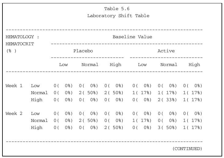
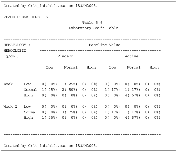
Laboratory Shift Table
Dataset
lb.txthas test measurements for various tests, each classified into low, normal, and high categoriesGoal: tabulate number and percentages of shifts (relative to baseline) at weeks 1 and 2
Read in data:
lb <- read.table("data/lb.txt", header = TRUE, na.strings = ".", stringsAsFactors = FALSE)
lb <- within(lb,
{
    lbnrind <- factor(lbnrind, levels = c("L", "N", "H"), labels = c("Low   ", "Normal", "High  "))
    week <- factor(week, levels = 0:2, labels = c("Baseline", "Week 1", "Week 2"))
})
str(lb)
'data.frame': 60 obs. of 9 variables:
$ subjid : int 101 101 101 101 101 101 102 102 102 102 ...
$ week : Factor w/ 3 levels "Baseline","Week 1",..: 1 2 3 1 2 3 1 2 3 1 ...
$ lbcat : chr "HEMATOLOGY" "HEMATOLOGY" "HEMATOLOGY" "HEMATOLOGY" ...
$ lbtest : chr "HEMATOCRIT" "HEMATOCRIT" "HEMATOCRIT" "HEMOGLOBIN" ...
$ lbstresu: chr "%" "%" "%" "g/dL" ...
$ lbstresn: num 31 39 44 11.5 13.2 14.3 39 39 44 11.5 ...
$ lbstnrlo: num 35 35 35 11.7 11.7 11.7 39 39 39 12.7 ...
$ lbstnrhi: num 49 49 49 15.9 15.9 15.9 52 52 52 17.2 ...
$ lbnrind : Factor w/ 3 levels "Low ","Normal",..: 1 2 2 1 2 2 2 2 2 1 ... subjid week lbcat lbtest lbstresu lbstresn lbstnrlo lbstnrhi lbnrind
1 101 Baseline HEMATOLOGY HEMATOCRIT % 31 35 49 Low
2 101 Week 1 HEMATOLOGY HEMATOCRIT % 39 35 49 Normal
3 101 Week 2 HEMATOLOGY HEMATOCRIT % 44 35 49 Normal
7 102 Baseline HEMATOLOGY HEMATOCRIT % 39 39 52 Normal
8 102 Week 1 HEMATOLOGY HEMATOCRIT % 39 39 52 Normal
9 102 Week 2 HEMATOLOGY HEMATOCRIT % 44 39 52 Normal
13 103 Baseline HEMATOLOGY HEMATOCRIT % 50 35 49 High
14 103 Week 1 HEMATOLOGY HEMATOCRIT % 39 35 49 Normal
15 103 Week 2 HEMATOLOGY HEMATOCRIT % 55 35 49 High
19 104 Baseline HEMATOLOGY HEMATOCRIT % 55 39 52 High
20 104 Week 1 HEMATOLOGY HEMATOCRIT % 45 39 52 Normal
21 104 Week 2 HEMATOLOGY HEMATOCRIT % 44 39 52 Normal
25 105 Baseline HEMATOLOGY HEMATOCRIT % 36 35 49 Normal
26 105 Week 1 HEMATOLOGY HEMATOCRIT % 39 35 49 Normal
27 105 Week 2 HEMATOLOGY HEMATOCRIT % 39 35 49 Normal
31 106 Baseline HEMATOLOGY HEMATOCRIT % 53 39 52 High
32 106 Week 1 HEMATOLOGY HEMATOCRIT % 50 39 52 Normal
33 106 Week 2 HEMATOLOGY HEMATOCRIT % 53 39 52 High
37 107 Baseline HEMATOLOGY HEMATOCRIT % 55 39 52 High
38 107 Week 1 HEMATOLOGY HEMATOCRIT % 56 39 52 High
39 107 Week 2 HEMATOLOGY HEMATOCRIT % 57 39 52 High
43 108 Baseline HEMATOLOGY HEMATOCRIT % 40 39 52 Normal
44 108 Week 1 HEMATOLOGY HEMATOCRIT % 53 39 52 High
45 108 Week 2 HEMATOLOGY HEMATOCRIT % 54 39 52 High
49 109 Baseline HEMATOLOGY HEMATOCRIT % 39 39 52 Normal
50 109 Week 1 HEMATOLOGY HEMATOCRIT % 53 39 52 High
51 109 Week 2 HEMATOLOGY HEMATOCRIT % 57 39 52 High
55 110 Baseline HEMATOLOGY HEMATOCRIT % 50 39 52 Normal
56 110 Week 1 HEMATOLOGY HEMATOCRIT % 51 39 52 Normal
57 110 Week 2 HEMATOLOGY HEMATOCRIT % 57 39 52 High The treatment assignments are available separately. As before, after reading in the data, we convert it to a named vector of treatment assignments.
treat <- read.table("data/treat-2.txt", header = TRUE, stringsAsFactors = FALSE)
treat <- within(treat,
{
    trtcd <- factor(trtcd, levels = c(0, 1), labels = c("Placebo", "Active"))
})
treat.trtcd <- structure(treat$trtcd,
                         names = as.character(treat$subjid)) # should be unique
treat.trtcd
101 102 103 104 105 106 107 108 109 110
Active Placebo Placebo Active Placebo Placebo Active Active Active Active
Levels: Placebo ActiveTo get the laboratory shift tables, we would ideally want a dataset with one row for each patient, and columns specifying baseline, week 1, and week 2 status. We can do this by splitting the lb data by patient, applying a function to each component to transform them into a single row, and recombining them using rbind().
Instead, just to illustrate a different approach, we will construct the laboratory shift table using a control flow more typical in structured imperative programming.
In the following function, lb contains the laboratory test data, and cat and test provide the lab category and test.
labshiftTable <- function(lb, all.trtcd, cat, test)
{
    x <- subset(lb, lbcat == cat & lbtest == test)
    makeName <- function(x, y) paste(y, x, sep = ".") # utility function
    ## available status categories
    uind <- levels(x$lbnrind)
    uweek <- levels(x$week) # first level is assumed to be Baseline
    utrt <- levels(all.trtcd)
    ans <- matrix(0,
                  nrow = length(uweek[-1]) * length(uind),
                  ncol = length(utrt) * length(uind),
                  dimnames = list(outer(uind, uweek[-1], makeName),
                                  outer(uind, utrt, makeName)))
    ## loop over subjects and accumulate counts
    for (i in unique(as.character(x$subjid)))
    {
        trtcd <- all.trtcd[i]
        baseline.status <- subset(x, subjid == i & week == uweek[1])[["lbnrind"]]
        ## for each week, compare to baseline
        for (w in uweek[-1])
        {
            week.status <- subset(x, subjid == i & week == w)[["lbnrind"]]
            row <- makeName(week.status, w)
            col <- makeName(baseline.status, trtcd)
            ans[row, col] <- ans[row, col] + 1
        }
    }
    ans
}
lst.hematocrit <- labshiftTable(lb, treat.trtcd, cat = "HEMATOLOGY", test = "HEMATOCRIT")
lst.hematocrit
Placebo.Low Placebo.Normal Placebo.High Active.Low Active.Normal Active.High
Week 1.Low 0 0 0 0 0 0
Week 1.Normal 0 2 2 1 1 1
Week 1.High 0 0 0 0 2 1
Week 2.Low 0 0 0 0 0 0
Week 2.Normal 0 2 0 1 0 1
Week 2.High 0 0 2 0 3 1To compute proportions, we need to divide by number of patients per treatment arm. This can be incorporated in the function above, but we will just do it manually here, as well as add some basic formatting.
ntotal <- table(treat.trtcd)
pct.hematocrit <- round(100 * lst.hematocrit / rep(ntotal, each = 2 * 3 * 3))
combined.hematocrit <-
    structure(sprintf("%2d (%3d%%)", lst.hematocrit, pct.hematocrit),
              dim = dim(lst.hematocrit))
combined.hematocrit <- cbind(c("Week 1", "", "", "Week 2", "", ""),
                             rep(levels(lb$lbnrind), 2),
                             combined.hematocrit)
combined.hematocrit <- rbind(c("HEMATOLOGY", "", "", "Active", "", "", "Placebo", ""),
                             c("HEMATOCRIT", "", rep("---------", 6)),
                             c("(%)       ", "", rep(levels(lb$lbnrind), 2)),
                             combined.hematocrit)
dimnames(combined.hematocrit) <- list(rep("", nrow(combined.hematocrit)),
                                      rep("", ncol(combined.hematocrit)))
print(combined.hematocrit, right = TRUE, quote = FALSE)
 HEMATOLOGY                     Active                       Placebo
 HEMATOCRIT        --------- --------- --------- --------- --------- ---------
 (%)                  Low       Normal    High      Low       Normal    High
     Week 1 Low     0 (  0%)  0 (  0%)  0 (  0%)  0 (  0%)  0 (  0%)  0 (  0%)
            Normal  0 (  0%)  2 ( 50%)  2 ( 50%)  1 ( 17%)  1 ( 17%)  1 ( 17%)
            High    0 (  0%)  0 (  0%)  0 (  0%)  0 (  0%)  2 ( 33%)  1 ( 17%)
     Week 2 Low     0 (  0%)  0 (  0%)  0 (  0%)  0 (  0%)  0 (  0%)  0 (  0%)
            Normal  0 (  0%)  2 ( 50%)  0 (  0%)  1 ( 17%)  0 (  0%)  1 ( 17%)
            High    0 (  0%)  0 (  0%)  2 ( 50%)  0 (  0%)  3 ( 50%)  1 ( 17%)
Incorporating these cosmetic updates into the labshiftTable() function is left as an exercise.
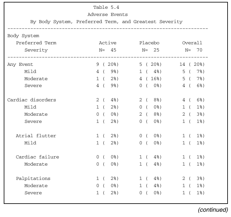
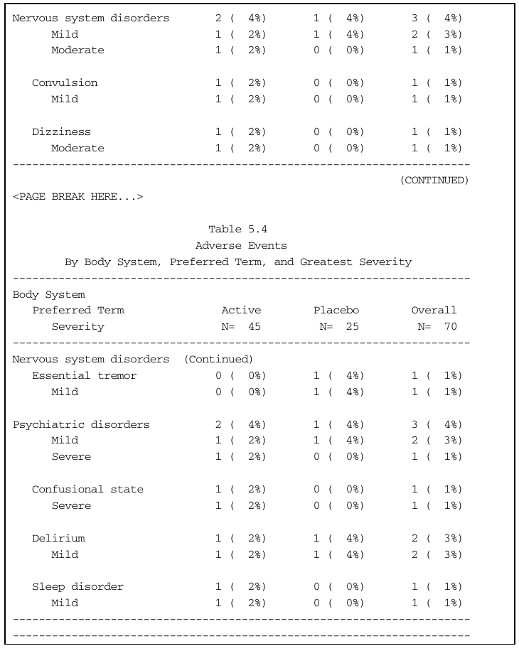
Summary of Adverse Events by Maximum Severity
- Read and pre-process data
treat <- read.table("data/treat-1.txt", header = TRUE, stringsAsFactors = FALSE)
treat <- transform(treat, trtcd = factor(trtcd, levels = c(1, 0), labels = c("Active", "Placebo")))
ae <- read.table("data/ae.txt", header = TRUE, stringsAsFactors = FALSE)
ae <-
    transform(ae,
              aerel = factor(aerel, levels = 1:3, labels = c("not", "possibly", "probably")),
              aesev = factor(aesev, levels = 1:3,
                             labels = c("Mild", "Moderate", "Severe"),
                             ordered = TRUE)) # so that 'maximum' makes sense
str(treat)
'data.frame': 70 obs. of 2 variables:
$ subjid: int 101 102 103 104 105 106 107 108 109 110 ...
$ trtcd : Factor w/ 2 levels "Active","Placebo": 1 2 2 1 2 2 1 1 2 1 ... subjid aerel aesev aebodsys aedecod
1 101 not Mild Cardiac disorders Atrial flutter
2 101 possibly Mild Gastrointestinal disorders Constipation
3 102 possibly Moderate Cardiac disorders Cardiac failure
4 102 not Mild Psychiatric disorders Delirium
5 103 not Mild Cardiac disorders Palpitations
6 103 not Moderate Cardiac disorders Palpitations
7 103 possibly Moderate Cardiac disorders Tachycardia
8 115 probably Moderate Gastrointestinal disorders Abdominal pain
9 115 probably Mild Gastrointestinal disorders Anal ulcer
10 116 possibly Mild Gastrointestinal disorders Constipation
11 117 possibly Moderate Gastrointestinal disorders Dyspepsia
12 118 probably Severe Gastrointestinal disorders Flatulence
13 119 not Severe Gastrointestinal disorders Hiatus hernia
14 130 not Mild Nervous system disorders Convulsion
15 131 possibly Moderate Nervous system disorders Dizziness
16 132 not Mild Nervous system disorders Essential tremor
17 135 not Severe Psychiatric disorders Confusional state
18 140 not Mild Psychiatric disorders Delirium
19 140 possibly Mild Psychiatric disorders Sleep disorder
20 141 not Severe Cardiac disorders PalpitationsNOTE: For example, subject 103 has two Palpitation events! How should these be counted?
The example we want to reproduce is an adverse even summary by maximum severity, which means
A patient should be counted only once at maximum severity within each subgrouping
Denominators should be the sum of all patients who had the given treatment
The summary table gives counts and percentages at various levels of hierarchy (all events, body system, event, severity).
We need to mainly work with the ae dataset, and require the treat dataset only to know the treatment assigned to each subject (and the number of patients by treatment arm). The two datasets are matched through the subjid column.
There are several ways to do the matching, all involving using subjid for (character) indexing. The simplest option here is to replace treat by a named vector giving treatment assignments.
treat.trtcd <- treat$trtcd
names(treat.trtcd) <- as.character(treat$subjid) # should be unique
treat.trtcd
101 102 103 104 105 106 107 108 109 110 111 112 113
Active Placebo Placebo Active Placebo Placebo Active Active Placebo Active Placebo Placebo Placebo
114 115 116 117 118 119 120 121 122 123 124 125 126
Active Placebo Active Placebo Active Active Active Active Placebo Active Placebo Active Active
127 128 129 130 131 132 133 134 135 136 137 138 139
Placebo Active Active Active Active Placebo Active Placebo Active Active Placebo Active Active
140 141 142 143 144 145 146 147 148 149 150 151 152
Active Active Placebo Active Placebo Active Active Placebo Active Active Active Active Placebo
153 154 155 156 157 158 159 160 161 162 163 164 165
Active Placebo Active Active Placebo Active Active Active Active Placebo Active Placebo Active
166 167 168 169 170
Active Placebo Active Active Active
Levels: Active PlaceboWe now need to create a summary table (using the same procedure) for various levels of hierarchy. As is typical when working with R, we will write a function to encapsulate a procedure we have to repeat multiple times. An alternative is to write a loop, but that usually makes code more difficult to maintain.
As input, this function will be provided a subset of the ae data after suitable subsetting by hierarchy, and a named vector of treatment assignments to be matched by subjid.
ae.summary.table <- function(x, all.trtcd)
{
    ## For each subjid, retain only the one with maximum severity.
    max.severity <-
        with(x, unlist(lapply(split(aesev, subjid),
                              max)))
    ## names of 'max.severity' are 'subjid'
    trtcd <- all.trtcd[ names(max.severity) ]
    tab <- table(max.severity, trtcd)
    tab[rowSums(tab) > 0, , drop = FALSE] # discard all-0 rows
}
Typical results at various levels of hierarchy:
            trtcd
max.severity Active Placebo
    Mild          4       1
    Moderate      1       4
Severe 4 0 trtcd
max.severity Active Placebo
Mild 1 0
Moderate 0 2
Severe 1 0ae.summary.table(subset(ae, aebodsys == "Cardiac disorders" & aedecod == "Palpitations"),
treat.trtcd) trtcd
max.severity Active Placebo
Moderate 0 1
Severe 1 0Next, we need to make some cosmetic additions such as row / column totals and percentages, for which we also need the number of patients. This is done using the following wrapper function, which also includes the option to name the top row (indicating hierarchy level).
ae.summary <- function(x, all.trtcd, ntot, label)
{
    tab <- ae.summary.table(x, all.trtcd)
    rownames(tab) <- paste0("      ", rownames(tab))
    tab <- cbind(tab, Overall = rowSums(tab))
    tab <- rbind(colSums(tab), tab)
    rownames(tab)[1] <- label
    prop.tab <- tab / rep( ntot, each = nrow(tab))
    s <- structure(sprintf("%2d (%3d%%)", tab, round(100 * prop.tab)),
                   dim = dim(tab),
                   dimnames = dimnames(tab))
    rbind(s, "") # blank line at end for formatting
}
With the additions, the “All Event” summary can be obtained as follows.
 Active Placebo Overall
45 25 70 Active Placebo Overall
Any Event 9 ( 20%) 5 ( 20%) 14 ( 20%)
Mild 4 ( 9%) 1 ( 4%) 5 ( 7%)
Moderate 1 ( 2%) 4 ( 16%) 5 ( 7%)
Severe 4 ( 9%) 0 ( 0%) 4 ( 6%)
We can now loop over all event types to construct combined table
all.ae <- ae.summary(ae, all.trtcd = treat.trtcd, ntot = ntotal, label = "Any Event")
for (bodsys in sort(unique(ae$aebodsys)))
{
    aesub <- subset(ae, aebodsys == bodsys)
    all.ae <-
        rbind(all.ae,
              ae.summary(aesub, ntot = ntotal, all.trtcd = treat.trtcd,
                         label = bodsys))
    for (decod in sort(unique(aesub$aedecod)))
    {
        all.ae <-
            rbind(all.ae,
                  ae.summary(subset(aesub, aedecod == decod),
                             ntot = ntotal, all.trtcd = treat.trtcd,
                             label = paste0("   ", decod)))
    }
}
print(rbind(sprintf("N = %2d", ntotal),
            "--------",
            all.ae),
      quote = FALSE)
Active Placebo Overall
N = 45 N = 25 N = 70
-------- -------- --------
Any Event 9 ( 20%) 5 ( 20%) 14 ( 20%)
Mild 4 ( 9%) 1 ( 4%) 5 ( 7%)
Moderate 1 ( 2%) 4 ( 16%) 5 ( 7%)
Severe 4 ( 9%) 0 ( 0%) 4 ( 6%)
Cardiac disorders 2 ( 4%) 2 ( 8%) 4 ( 6%)
Mild 1 ( 2%) 0 ( 0%) 1 ( 1%)
Moderate 0 ( 0%) 2 ( 8%) 2 ( 3%)
Severe 1 ( 2%) 0 ( 0%) 1 ( 1%)
Atrial flutter 1 ( 2%) 0 ( 0%) 1 ( 1%)
Mild 1 ( 2%) 0 ( 0%) 1 ( 1%)
Cardiac failure 0 ( 0%) 1 ( 4%) 1 ( 1%)
Moderate 0 ( 0%) 1 ( 4%) 1 ( 1%)
Palpitations 1 ( 2%) 1 ( 4%) 2 ( 3%)
Moderate 0 ( 0%) 1 ( 4%) 1 ( 1%)
Severe 1 ( 2%) 0 ( 0%) 1 ( 1%)
Tachycardia 0 ( 0%) 1 ( 4%) 1 ( 1%)
Moderate 0 ( 0%) 1 ( 4%) 1 ( 1%)
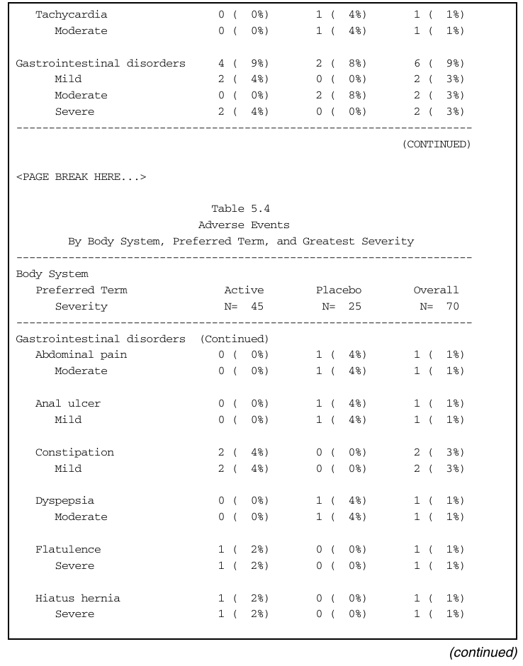
Gastrointestinal disorders 4 ( 9%) 2 ( 8%) 6 ( 9%)
Mild 2 ( 4%) 0 ( 0%) 2 ( 3%)
Moderate 0 ( 0%) 2 ( 8%) 2 ( 3%)
Severe 2 ( 4%) 0 ( 0%) 2 ( 3%)
Abdominal pain 0 ( 0%) 1 ( 4%) 1 ( 1%)
Moderate 0 ( 0%) 1 ( 4%) 1 ( 1%)
Anal ulcer 0 ( 0%) 1 ( 4%) 1 ( 1%)
Mild 0 ( 0%) 1 ( 4%) 1 ( 1%)
Constipation 2 ( 4%) 0 ( 0%) 2 ( 3%)
Mild 2 ( 4%) 0 ( 0%) 2 ( 3%)
Dyspepsia 0 ( 0%) 1 ( 4%) 1 ( 1%)
Moderate 0 ( 0%) 1 ( 4%) 1 ( 1%)
Flatulence 1 ( 2%) 0 ( 0%) 1 ( 1%)
Severe 1 ( 2%) 0 ( 0%) 1 ( 1%)
Hiatus hernia 1 ( 2%) 0 ( 0%) 1 ( 1%)
Severe 1 ( 2%) 0 ( 0%) 1 ( 1%)
Nervous system disorders 2 ( 4%) 1 ( 4%) 3 ( 4%)
Mild 1 ( 2%) 1 ( 4%) 2 ( 3%)
Moderate 1 ( 2%) 0 ( 0%) 1 ( 1%)
Convulsion 1 ( 2%) 0 ( 0%) 1 ( 1%)
Mild 1 ( 2%) 0 ( 0%) 1 ( 1%)
Dizziness 1 ( 2%) 0 ( 0%) 1 ( 1%)
Moderate 1 ( 2%) 0 ( 0%) 1 ( 1%)
Essential tremor 0 ( 0%) 1 ( 4%) 1 ( 1%)
Mild 0 ( 0%) 1 ( 4%) 1 ( 1%)
Psychiatric disorders 2 ( 4%) 1 ( 4%) 3 ( 4%)
Mild 1 ( 2%) 1 ( 4%) 2 ( 3%)
Severe 1 ( 2%) 0 ( 0%) 1 ( 1%)
Confusional state 1 ( 2%) 0 ( 0%) 1 ( 1%)
Severe 1 ( 2%) 0 ( 0%) 1 ( 1%)
Delirium 1 ( 2%) 1 ( 4%) 2 ( 3%)
Mild 1 ( 2%) 1 ( 4%) 2 ( 3%)
Sleep disorder 1 ( 2%) 0 ( 0%) 1 ( 1%)
Mild 1 ( 2%) 0 ( 0%) 1 ( 1%)
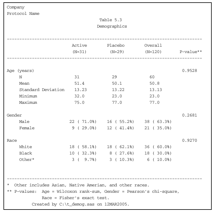
Demographic summary table
The goal is to reproduce the following report from the demog.txt data.
The original data contains a "." indicating a missing value. The data are read into R as follows.
demog <- read.table("data/demog.txt", header = TRUE, na.strings = ".", stringsAsFactors = FALSE)
demog <- within(demog,
{
    trt = factor(trt, levels = c(1, 0), labels = c("Active", "Placebo"))
    gender = factor(gender, levels = c(1, 2), labels = c("Male", "Female"))
    race = factor(race, levels = c(1, 2, 3), labels = c("White", "Black", "Other*"))
})
str(demog)
'data.frame': 60 obs. of 5 variables:
$ subjid: int 101 102 103 104 105 106 201 202 203 204 ...
$ trt : Factor w/ 2 levels "Active","Placebo": 2 1 1 2 1 2 1 2 1 2 ...
$ gender: Factor w/ 2 levels "Male","Female": 1 2 1 2 1 2 1 2 1 2 ...
$ race : Factor w/ 3 levels "White","Black",..: 3 1 2 1 3 1 3 1 2 1 ...
$ age : int 37 65 32 23 44 49 35 50 49 60 ...The contents of the summary table are all things we already know how to obtain, so the only difficulty here is to arrange the information in a suitable format.
Tests of independence
The report we wish to reproduce essentially contains three sets of tables, each summarizing the dependence of one demographic variable (age, gender, race) on treatment. This summary is in terms of a test for independence of the demographic attribute and the treatment assignment, and a comparative summary of the distributions.
The tests can be performed in R as follows.
The Wilcoxon rank-sum test is used for age vs treatment.
Warning in wilcox.test.default(x = c(65L, 32L, 44L, 35L, 49L, 39L, 67L, : cannot compute exact p-value with
tiesList of 7
$ statistic : Named num 445
..- attr(*, "names")= chr "W"
$ parameter : NULL
$ p.value : num 0.953
$ null.value : Named num 0
..- attr(*, "names")= chr "location shift"
$ alternative: chr "two.sided"
$ method : chr "Wilcoxon rank sum test with continuity correction"
$ data.name : chr "age by trt"
- attr(*, "class")= chr "htest"[1] 0.9527506Only the p-value is included in the report.
The test used for Gender is the χ2 test for contingency tables.
    Pearson's Chi-squared test with Yates' continuity correction

data:  xtabs(~gender + trt, data = demog)
X-squared = 0.69763, df = 1, p-value = 0.4036
For consistency with the SAS code, Yate’s continuity correction is not applied.
[1] 0.2680754Finally, the test used for race is Fisher’s exact test.
[1] 0.9269529Comparative summary
The numeric covariate age is summarized in the report by the number of observations, mean, standard deviation, minimum, and maximum. There is no built-in function in R to calculate exactly this set of summary statistics (although summary() is similar in spirit), so we define a function of our own.
univariate <- function(x)
{
    c("     N" = length(x),
      "     Mean" = mean(x, na.rm = TRUE),
      "     Standard Deviation" = sd(x, na.rm = TRUE),
      "     Minimum" = min(x, na.rm = TRUE),
      "     Maximum" = max(x, na.rm = TRUE))
}
This can be used to generate summaries for the relevant data subgroups, for example:
                      N                    Mean      Standard Deviation                 Minimum
               31.00000                51.35484                13.22762                32.00000
                Maximum
               75.00000
As we would like to present these three sets of summaries as columns in a matrix, we can “bind” them as columns to create a 3-column matrix.
age.summary <- with(demog,
                    cbind(Active = univariate(age[trt == "Active"]),
                          Placebo = univariate(age[trt == "Placebo"]),
                          Overall = univariate(age)))
age.summary
Active Placebo Overall
N 31.00000 29.00000 60.0000
Mean 51.35484 50.10345 50.7500
Standard Deviation 13.22762 13.22429 13.1286
Minimum 32.00000 23.00000 23.0000
Maximum 75.00000 77.00000 77.0000This is unfortunately not formatted as nicely as we would like when printed. We may eventually have to do a lot more work to combine multiple tables, but for now we can use the formatC() function to get something more presentable.
                        Active Placebo Overall
     N                  31     29      60
     Mean               51.35  50.1    50.75
     Standard Deviation 13.23  13.22   13.13
     Minimum            32     23      23
     Maximum            75     77      77
One drawback of this approach is that we have to know the number of treatment arms and their exact names. An alternative is to write a function to do this automatically.
In addition to the two treatment arms, We also want to include a summary for the overall data. The SAS code takes the somewhat odd approach of duplicating the whole dataset and artificially marking the second copy as the “overall” treatment arm. Presumably, this is to make use of built-in summary by group procedures.
R is a fully featured programming language where we can write our own functions, so this kind of artificial duplication is unnecessary. Our function has an optional argument that allows the overall summary to be included or excluded. It also allows customizing the summary procedure as well as the test of independence used.
summarizeByTreatment <-
    function(x, t, summaryFun = summary,
             test = c("none", "wilcox", "anova", "fisher", "chisq"),
             overall = TRUE, overall.label = "Overall")
    {
        if (is.character(test)) test <- match.arg(test)
        xlist <- split(x, t)
        slist <- lapply(xlist, summaryFun)
        if (overall) {
            olist <- list(summaryFun(x))
            names(olist) <- overall.label
            slist <- c(slist, olist)
        }
        ans <- do.call(cbind, slist)
        if (is.function(test)) {
            test.out <- test(x, t)
        }
        else {
            test.out <-
                switch(test,
                       wilcox = wilcox.test(x ~ t)$p.value,
                       anova = anova(aov(x ~ t))$"Pr(>F)"[1],
                       fisher = fisher.test(table(x, t))$p.value,
                       chisq = chisq.test(table(x, t))$p.value,
                       NULL)
        }
        attr(ans, "test") <- test
        attr(ans, "pvalue") <- test.out
        ans
    }
The attr(*, *) represents arbitrary information that can be attached to any R object as “attributes”.
The following examples illustrate various ways to use this function to produce different variants of comparative summary tables.
age.summary <-
    with(demog,
         summarizeByTreatment(age, trt, summaryFun = univariate, test = "wilcox"))
Warning in wilcox.test.default(x = c(65L, 32L, 44L, 35L, 49L, 39L, 67L, : cannot compute exact p-value with
ties Active Placebo Overall
N 31 29 60
Mean 51.35 50.1 50.75
Standard Deviation 13.23 13.22 13.13
Minimum 32 23 23
Maximum 75 77 77
attr(,"test")
[1] wilcox
attr(,"pvalue")
[1] 0.9527506race.summary <-
with(demog,
summarizeByTreatment(race, trt, summaryFun = table, test = "fisher"))
print(formatC(race.summary, width = 2), quote = FALSE) Active Placebo Overall
White 18 18 36
Black 10 8 18
Other* 3 3 6
attr(,"test")
[1] fisher
attr(,"pvalue")
[1] 0.9269529The next example shows how a user-defined test function can be used instead of the built-in alternatives. This is easy because in R, functions can be passed on as arguments to other functions.
my.chisq.test <- function(x, t)
{
    chisq.test(table(x, t), correct = FALSE)$p.value
}
gender.summary <-
    with(demog,
         summarizeByTreatment(gender, trt, summaryFun = table,
                              test = my.chisq.test))
print(formatC(gender.summary, width = 2), quote = FALSE)
Active Placebo Overall
Male 22 16 38
Female 9 12 21
attr(,"test")
function(x, t)
{
chisq.test(table(x, t), correct = FALSE)$p.value
}
attr(,"pvalue")
[1] 0.2680754Categorical variables are summarized by frequency tables (as produced by the built-in table() function) in the examples shown above. However, we want to include the percentages as well. This again requires a custom function to be defined.
tableWithPercent <- function(f)
{
    tab <- table(f)
    prop <- prop.table(tab)
    structure(sprintf("%4d (%5.1f%%)", tab, 100*prop),
              names = sprintf("     %s", names(tab)))
}
This can be used as follows.
race.summary <-
    with(demog,
         summarizeByTreatment(race, trt, summaryFun = tableWithPercent,
                              test = "fisher"))
print(race.summary, quote = FALSE)
Active Placebo Overall
White 18 ( 58.1%) 18 ( 62.1%) 36 ( 60.0%)
Black 10 ( 32.3%) 8 ( 27.6%) 18 ( 30.0%)
Other* 3 ( 9.7%) 3 ( 10.3%) 6 ( 10.0%)
attr(,"test")
[1] fisher
attr(,"pvalue")
[1] 0.9269529gender.summary <-
with(demog,
summarizeByTreatment(gender, trt, summaryFun = tableWithPercent,
test = my.chisq.test))
print(gender.summary, quote = FALSE) Active Placebo Overall
Male 22 ( 71.0%) 16 ( 57.1%) 38 ( 64.4%)
Female 9 ( 29.0%) 12 ( 42.9%) 21 ( 35.6%)
attr(,"test")
function(x, t)
{
chisq.test(table(x, t), correct = FALSE)$p.value
}
<bytecode: 0x55cdddca3a30>
attr(,"pvalue")
[1] 0.2680754We now have all the calculations necessary to reproduce the table. All that remains is to present them together in a suitable format.
Combining individual pieces to produce overall table
It is of course possible to exactly reproduce the table, including exact formats and widths, but this would involve tedious work unless absolutely necessary.
The next best approximation is to recreate a matrix combining the three tables along with the p-values for the tests of independence. For this, we can first write a function that incorporates the p-values in the table, to be combined later.
addPValue <- function(x, label = "")
{
    pvalue <- attr(x, "pvalue")
    d <- dim(x)
    ans <- rbind("", cbind(x, "  P-value**" = ""))
    rownames(ans)[1] <- label
    ans[1, d[2]+1] <- formatC(pvalue, digits = 4, width = 9, format = "f")
    ## attributes(ans) <- NULL
    ans
}
This is used, for example, to extend the table for race as follows.
            Active          Placebo         Overall           P-value**
            ""              ""              ""              "   0.9270"
     White  "  18 ( 58.1%)" "  18 ( 62.1%)" "  36 ( 60.0%)" ""
     Black  "  10 ( 32.3%)" "   8 ( 27.6%)" "  18 ( 30.0%)" ""
     Other* "   3 (  9.7%)" "   3 ( 10.3%)" "   6 ( 10.0%)" ""
These can be combined, with blank lines as desired, using rbind().
age.summary.text <- formatC(age.summary)
print(
    rbind("", addPValue(age.summary.text, label = "Age (years)"),
          "", addPValue(gender.summary, label = "Gender"),
          "", addPValue(race.summary, label = "Race"),
          "", "", "")
, quote = FALSE)
Active Placebo Overall P-value**
Age (years) 0.9528
N 31 29 60
Mean 51.35 50.1 50.75
Standard Deviation 13.23 13.22 13.13
Minimum 32 23 23
Maximum 75 77 77
Gender 0.2681
Male 22 ( 71.0%) 16 ( 57.1%) 38 ( 64.4%)
Female 9 ( 29.0%) 12 ( 42.9%) 21 ( 35.6%)
Race 0.9270
White 18 ( 58.1%) 18 ( 62.1%) 36 ( 60.0%)
Black 10 ( 32.3%) 8 ( 27.6%) 18 ( 30.0%)
Other* 3 ( 9.7%) 3 ( 10.3%) 6 ( 10.0%)
Further adjustments, such as padding texts for better alignment, can be also done.
age.summary.text[] <- paste0("    ", age.summary.text)
trt.counts <- with(demog, c(table(trt), length(trt)))
combined.table <-
    rbind(c(sprintf("   (N=%d)", trt.counts), ""),
          "", addPValue(age.summary.text, label = "Age (years)"),
          "", addPValue(gender.summary, label = "Gender"),
          "", addPValue(race.summary, label = "Race"),
          "", "", "")
colnames(combined.table)[1:3] <- paste0("   ", colnames(combined.table)[1:3])
print(combined.table, quote = FALSE)
Active Placebo Overall P-value**
(N=31) (N=29) (N=60)
Age (years) 0.9528
N 31 29 60
Mean 51.35 50.1 50.75
Standard Deviation 13.23 13.22 13.13
Minimum 32 23 23
Maximum 75 77 77
Gender 0.2681
Male 22 ( 71.0%) 16 ( 57.1%) 38 ( 64.4%)
Female 9 ( 29.0%) 12 ( 42.9%) 21 ( 35.6%)
Race 0.9270
White 18 ( 58.1%) 18 ( 62.1%) 36 ( 60.0%)
Black 10 ( 32.3%) 8 ( 27.6%) 18 ( 30.0%)
Other* 3 ( 9.7%) 3 ( 10.3%) 6 ( 10.0%)
To add the required headers and footers (and horizontal lines), it is probably easiest to capture the output above as text and append free-form text as necessary.
combined.table.text <- capture.output(print(combined.table, quote = FALSE))
head(combined.table.text)
[1] " Active Placebo Overall P-value**"
[2] " (N=31) (N=29) (N=60) "
[3] " "
[4] "Age (years) 0.9528 "
[5] " N 31 29 60 "
[6] " Mean 51.35 50.1 50.75 "width <- max(nchar(combined.table.text)) # actually all equal
hr <- paste(rep("-", width), collapse = "")
combined.table.updated <-
c("Company",
"Protocol name",
" Table x.x",
" Demographics",
"",
hr, combined.table.text[c(1, 2)], hr, combined.table.text[-c(1,2)], hr,
"* Other includes Asian, Native American, and other races",
"** P-values: Age = Wilcoxon rank-sum, Gender = Pearson's chi-square,",
" Race = Fisher's exact test.",
"")
cat(combined.table.updated, sep = "\n")Company
Protocol name
Table x.x
Demographics
-----------------------------------------------------------------------------
Active Placebo Overall P-value**
(N=31) (N=29) (N=60)
-----------------------------------------------------------------------------
Age (years) 0.9528
N 31 29 60
Mean 51.35 50.1 50.75
Standard Deviation 13.23 13.22 13.13
Minimum 32 23 23
Maximum 75 77 77
Gender 0.2681
Male 22 ( 71.0%) 16 ( 57.1%) 38 ( 64.4%)
Female 9 ( 29.0%) 12 ( 42.9%) 21 ( 35.6%)
Race 0.9270
White 18 ( 58.1%) 18 ( 62.1%) 36 ( 60.0%)
Black 10 ( 32.3%) 8 ( 27.6%) 18 ( 30.0%)
Other* 3 ( 9.7%) 3 ( 10.3%) 6 ( 10.0%)
-----------------------------------------------------------------------------
* Other includes Asian, Native American, and other races
** P-values: Age = Wilcoxon rank-sum, Gender = Pearson's chi-square,
Race = Fisher's exact test.Alternative presentations
There are many alternatives to plain ASCII tables, and R has good support for PDF through LaTeX and various other formats, including HTML, through markdown.
The following is an example of how the table above could be formatted in markdown. This is produced using the pander package in R, meant to work with a specific variant of markdown supported by the pandoc software. The output is essentially formatted as a text table.
library(pander)
combined.table.md <- format(combined.table[1:17, ])
colnames(combined.table.md)[1:3] <-
    sprintf("%s\\\n%s", colnames(combined.table.md)[1:3], combined.table.md[1,1:3])
combined.table.md <- combined.table.md[-c(1,2), ] # drop unneeded rows
pandoc.table(combined.table.md, justify = "left", emphasize.rownames = FALSE,
             style = "multiline", keep.line.breaks = TRUE)
--------------------------------------------------------------------------
                Active\       Placebo\      Overall\      P-value**
                     (N=31)        (N=29)        (N=60)
-------------------- ------------- ------------- ------------- -----------
Age (years)                                                    0.9528

N                    31            29            60

Mean                 51.35         50.1          50.75

Standard Deviation   13.23         13.22         13.13

Minimum              32            23            23

Maximum              75            77            77


Gender                                                         0.2681

Male                 22 ( 71.0%)   16 ( 57.1%)   38 ( 64.4%)

Female               9 ( 29.0%)    12 ( 42.9%)   21 ( 35.6%)


Race                                                           0.9270

White                18 ( 58.1%)   18 ( 62.1%)   36 ( 60.0%)

Black                10 ( 32.3%)   8 ( 27.6%)    18 ( 30.0%)

Other*               3 ( 9.7%)     3 ( 10.3%)    6 ( 10.0%)
--------------------------------------------------------------------------
Such markdown tables can be easily converted into HTML tables, such as the one below:
## replace all spaces by non-breaking spaces for formatting
combined.table.md[] <- gsub(" ", " ", combined.table.md, fixed = TRUE)
combined.table.md[] <- paste0("`", combined.table.md, "`")
combined.table.md[combined.table.md == "``"] <- " "
rownames(combined.table.md)[c(1, 8, 12)] <-
sprintf("__%s__", rownames(combined.table.md)[c(1, 8, 12)])
rownames(combined.table.md)[-c(1, 8, 12)] <-
gsub(" ", " ", rownames(combined.table.md)[-c(1, 8, 12)], fixed = TRUE)pandoc.table(combined.table.md, emphasize.rownames = FALSE,
justify = rep(c("left", "center"), c(1, ncol(combined.table.md))),
keep.line.breaks = TRUE, split.tables = 120,
caption = "Demographic table. * Other includes Asian, Native American, and other races.
** P-values: Age = Wilcoxon rank-sum, Gender = Pearson's chi-square,
Race = Fisher's exact test.")| Active (N=31) |
Placebo (N=29) |
Overall (N=60) |
P-value** | |
|---|---|---|---|---|
| Age (years) | |
|
|
0.9528 |
| N | 31 |
29 |
60 |
|
| Mean | 51.35 |
50.1 |
50.75 |
|
| Standard Deviation | 13.23 |
13.22 |
13.13 |
|
| Minimum | 32 |
23 |
23 |
|
| Maximum | 75 |
77 |
77 |
|
|
|
|
|
|
| Gender | |
|
|
0.2681 |
| Male | 22 ( 71.0%) |
16 ( 57.1%) |
38 ( 64.4%) |
|
| Female | 9 ( 29.0%) |
12 ( 42.9%) |
21 ( 35.6%) |
|
|
|
|
|
|
| Race | |
|
|
0.9270 |
| White | 18 ( 58.1%) |
18 ( 62.1%) |
36 ( 60.0%) |
|
| Black | 10 ( 32.3%) |
8 ( 27.6%) |
18 ( 30.0%) |
|
| Other* | 3 ( 9.7%) |
3 ( 10.3%) |
6 ( 10.0%) |
|
As we have seen, markdown documents can be converted into various other formats.