Penalized Regression
Deepayan Sarkar
Penalized regression
Another potential remedy for collinearity
Decreases variability of estimated coefficients at the cost of introducing bias
Also known as regularization
Important beyond the collinearity context
Certain types of penalties can be used for variable selection in a natural way
Penalized regression provides solutions in ill-posed (rank-deficient) problems
Familiar examples of such models are ANOVA models with all dummy variables
A more realistic situation is models with \(p > n\) (more covariates than observations)
Penalized likelihood and Bayesian interpretation
We have already seen an example of penalized regression: smoothing splines
Given data \(\{ (x_i, y_i ) : x_i \in [a, b] \}\), goal is to find \(f\) that minimizes (given \(\lambda > 0\))
\[ \sum_i (y_i - f(x_i))^2 + \lambda \int_{a}^{b} (f^{\prime\prime}(t))^2 dt \]
The solution is a natural cubic spline
Here \(f\) is the parameter of interest
The (ill-posed) least squares problem is regularized by adding a penalty for “undesirable” (wiggly) solutions
The same idea can be applied for usual (finite-dimensional) parameters as well
Penalized likelihood and Bayesian interpretation
Penalized regression is a special case of the more general penalized likelihood approach
This is easiest to motivate using a Bayesian argument
Consider unknown parameter \(\theta\) and observed data \(y\) with
- Bayesian inference is based on the posterior distribution of \(\theta\), given by
\[ p(\theta | y) = \frac{p(\theta, y)}{p(y)} = \frac{p(\theta) \, p(y | \theta)}{p(y)} \]
- Here \(p(y)\) is the marginal density of \(y\) given by
\[ p(y) = \int p(\theta) \, p(y | \theta) \, d\theta \]
Penalized likelihood and Bayesian interpretation
How does posterior \(p(\theta | y)\) lead to inference on \(\theta\)?
We could look at \(E(\theta | y)\), \(V(\theta | y)\), etc.
We could also look at the maximum-a-posteriori (MAP) estimator
\[ \hat\theta = \arg \max_{\theta} p(\theta | y) \]
- This is analagous to MLE in the classical frequentist setup
Unfortunately, \(p(y)\) is in general difficult to compute
This has led to methods to simulate from \(p(\theta | y)\) without knowing \(p(y)\) (MCMC)
Penalized likelihood and Bayesian interpretation
Fortunately, MAP estimation does not require \(p(y)\), which does not depend on \(\theta\)
\(\hat\theta\) is given by
The first term is precisely the usual log-likelihood
The second term can be viewed as a “regularization penalty” for “undesirable” \(\theta\)
Penalized regression: normal linear model with normal prior
- Assume the usual normal linear model
\[ \mathbf{y} | \mathbf{X}, \beta \sim N( \mathbf{X} \beta, \sigma^2 \mathbf{I}) \]
- Addidionally, assume an i.i.d. mean-zero normal prior for each \(\beta_j\)
\[ \beta \sim N( \mathbf{0}, \tau^2 \mathbf{I}) \]
- Then it is easy to see that if \(L\) is the penalized log-likelihood, then
\[ -2 L(\beta) = C(\sigma^2, \tau^2) + \frac{1}{\sigma^2} \sum_{i=1}^n (y_i - \mathbf{x}_i^T \beta)^2 + \frac{1}{\tau^2} \sum_{j=1}^p \beta_j^2 \]
- Thus, the MAP estimate of \(\beta\) is (as a function of the unknown \(\sigma^2\) and “prior parameter” \(\tau^2\))
\[ \hat\beta = \arg \min_{\beta}\, \sum_{i=1}^n (y_i - \mathbf{x}_i^T \beta)^2 + \frac{\sigma^2}{\tau^2} \sum_{j=1}^p \beta_j^2 \]
Ridge regression
- This is known as Ridge regression, with the problem defined in terms of the “tuning parameter” \(\lambda\)
\[ \hat\beta = \arg \min_{\beta}\, \sum_{i=1}^n (y_i - \mathbf{x}_i^T \beta)^2 + \lambda \sum_{j=1}^p \beta_j^2 \]
As discussed earlier, this approach does not really make sense unless columns of \(\mathbf{X}\) are standardized
It is also not meaningful to penalize the intercept
For these reasons, in what follows, we assume without loss of generality that
Columns of \(\mathbf{X}\) have been centered and scaled to have mean \(0\) and variance \(1\)
\(\mathbf{y}\) has been centered to have mean 0
The model is fit without an intercept (which is separately estimated as \(\bar{y}\))
In practice, these issues are usually handled by model fitting software in the background
Ridge regression: solution
- It is easy to see that the objective function to be minimized is
\[ \mathbf{y}^T \mathbf{y} + \beta^T \mathbf{X}^T \mathbf{X} \beta - 2 \mathbf{y}^T \mathbf{X} \beta + \lambda \beta^T \beta = \mathbf{y}^T \mathbf{y} + \beta^T (\mathbf{X}^T \mathbf{X} + \lambda \mathbf{I}) \beta - 2 \mathbf{y}^T \mathbf{X} \beta \]
- The corresponding normal equations are
\[ (\mathbf{X}^T \mathbf{X} + \lambda \mathbf{I}) \beta = \mathbf{X}^T \mathbf{y} \]
- This gives the Ridge estimator
\[ \hat{\beta} = (\mathbf{X}^T \mathbf{X} + \lambda \mathbf{I})^{-1} \mathbf{X}^T \mathbf{y} \]
Note that \(\mathbf{X}^T \mathbf{X} + \lambda \mathbf{I}\) is always invertible
To prove this, use the singular value decomposition of \(\mathbf{X}^T \mathbf{X} = \mathbf{A} \mathbf{\Lambda} \mathbf{A}^T\)
\[ \mathbf{X}^T \mathbf{X} + \lambda \mathbf{I} = \mathbf{A} (\mathbf{\Lambda} + \lambda \mathbf{I}) \mathbf{A}^T \]
- Even if \(\mathbf{\Lambda}\) has some zero diagonal entries, all diagonal entries of \(\mathbf{\Lambda} + \lambda \mathbf{I}\) are at least \(\lambda\)
Ridge regression: solution
As \(\lambda \to 0\), \(\hat{\beta}_{ridge} \to \hat{\beta}_{OLS}\)
As \(\lambda \to \infty\), \(\hat{\beta}_{ridge} \to \mathbf{0}\)
In the special case where columns of \(\mathbf{X}\) are orthogonal (\(\mathbf{A} = \mathbf{I}\))
\[ \hat{\beta}_{ridge} = \frac{1}{1+\lambda} \hat{\beta}_{OLS} \]
This illustates the essential feature of ridge regression: shrinkage towards \(0\) (the prior mean of \(\beta\))
The ridge penalty introduces bias by shrinkage but reduces variance
Ridge regression in the presence of collinearity
- Recall our experiment with simulated collinearity
simCollinear <- function(n = 100)
{
    z1 <- rnorm(n)
    z2 <- rnorm(n)
    x1 <- z1 + z2 + 0.1 * rnorm(n)
    x2 <- z1 - 2 * z2 + 0.1 * rnorm(n)
    x3 <- 2 * z1 - z2 + 0.1 * rnorm(n)
    y <- x1 + 2 * x2 + 2 * rnorm(n) # x3 has coefficient 0
    data.frame(y, x1, x2, x3)
}
d3 <- simCollinear()
lm(y ~ . , data = d3)
Call:
lm(formula = y ~ ., data = d3)

Coefficients:
(Intercept)           x1           x2           x3
    -0.3256       0.7419       1.8612       0.1909
Ridge regression in the presence of collinearity
                   x1         x2         x3
-0.3339996 0.1511181 1.2421567 0.7907122 x1 x2 x3
-0.34263086 0.01199235 1.03851408 0.89352016
## Replicate this several times
sim.results <-
    replicate(100,
    {
        d3 <- simCollinear()
        beta.ols <- coef(lm(y ~ . , data = d3))[-1]
        beta.ridge.1 <- coef(lm.ridge(y ~ . , data = d3, lambda = 1))[-1]
        beta.ridge.10 <- coef(lm.ridge(y ~ . , data = d3, lambda = 10))[-1]
        data.frame(beta1 = c(beta.ols[1], beta.ridge.1[1], beta.ridge.10[1]),
                   beta2 = c(beta.ols[2], beta.ridge.1[2], beta.ridge.10[2]),
                   beta3 = c(beta.ols[3], beta.ridge.1[3], beta.ridge.10[3]),
                   which = c("lambda=0 (OLS)", "lambda=1", "lambda=10"))
    }, simplify = FALSE)
sim.df <- do.call(rbind, sim.results)
Ridge regression in the presence of collinearity
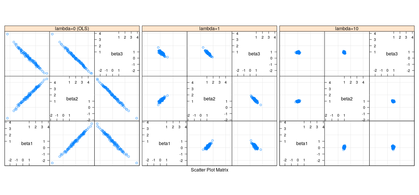
Bias and variance of Ridge regression
- Recall that true \(\beta = (1, 2, 0)\)
with(sim.df, rbind(tapply(beta1, which, mean),
                   tapply(beta2, which, mean),
                   tapply(beta3, which, mean)))
lambda=0 (OLS) lambda=1 lambda=10
[1,] 1.024926051 0.2217080 0.04698428
[2,] 1.997629453 1.1864466 0.96557666
[3,] -0.005341892 0.7949516 0.92124664 lambda=0 (OLS) lambda=1 lambda=10
[1,] 1.163054 0.2630750 0.11957701
[2,] 1.174441 0.2519598 0.07013490
[3,] 1.171263 0.2512505 0.08062144Bias and variance of Ridge regression
- The variance of the ridge estimator is
\[ V(\hat\beta) = \sigma^2 \mathbf{W} \mathbf{X}^T \mathbf{X} \mathbf{W} \quad \text{where} \quad \mathbf{W} = (\mathbf{X}^T \mathbf{X} + \lambda \mathbf{I})^{-1} \]
- The expectation of the ridge estimator is
\[ E(\hat\beta) = \mathbf{W} \mathbf{X}^T \mathbf{X} \beta \]
- The bias of the ridge estimator is
\[ \text{bias}(\hat\beta) = (\mathbf{W} \mathbf{X}^T \mathbf{X} - \mathbf{I}) \beta = -\lambda \mathbf{W} \beta \]
- This follows because
\[ \mathbf{W} (\mathbf{X}^T \mathbf{X} + \lambda \mathbf{I}) = \mathbf{I} \implies \mathbf{W} \mathbf{X}^T \mathbf{X} - \mathbf{I} = \lambda \mathbf{W} \]
Bias and variance of Ridge regression
It can be shown that
- the total variance \(\sum_j V(\hat{\beta}_j)\) is monotone decreasing w.r.t. \(\lambda\)
- the total squared bias \(\sum_j \text{bias}^2(\hat{\beta}_j)\) is monotone increasing w.r.t. \(\lambda\)
It can also be shown that there exists some \(\lambda\) for which the total MSE of \(\hat{\beta}\) is less than the MSE of \(\hat{\beta}_{OLS}\)
This is a surprising result that is an instance of a more general phenomenon in decision theory
Note however that the total MSE has no useful interpretation for the overall fit
We still need to address the problem of choosing \(\lambda\)
Before doing so, let us consider a related (but much more interesting) estimator called LASSO
LASSO
LASSO stands for “Least Absolute Shrinkage and Selection Operator”
The LASSO estimator is given by solving a penalized regression with a \(L_1\) penalty (rather than \(L_2\))
\[ \hat\beta = \arg \min_{\beta} \quad \frac{1}{2} \sum_{i=1}^n (y_i - \mathbf{x}_i^T \beta)^2 + \lambda \sum_{j=1}^p \lvert \beta_j \rvert \]
This corresponds to an i.i.d. double exponential prior on each \(\beta_j\)
Even though the change seems subtle, the behaviour of the estimator changes dramatically
The problem is much more difficult to solve numerically (except when \(\mathbf{X}\) is orthogonal — exercise)
It is an area of active research, and implementations have improved considerably over the last few decades
We will not go into further theoretical details, but only look at some practical aspects
LASSO in the presence of collinearity
library(glmnet) # usage: glmnet(X, y, alpha, ...)
coef(with(d3, glmnet(cbind(x1, x2, x3), y, alpha = 1, lambda = 1)))
4 x 1 sparse Matrix of class "dgCMatrix"
s0
(Intercept) -0.3733872
x1 .
x2 0.8227224
x3 0.6775433
## Replicate this several times
sim.results.lasso <-
    replicate(100,
    {
        d3 <- simCollinear()
        beta.ols <- coef(lm(y ~ . , data = d3))[-1]
        fm.lasso <- with(d3, glmnet(cbind(x1, x2, x3), y, alpha = 1, lambda = c(2, 1)))
        beta.lasso <- as.matrix(coef(fm.lasso))[-1, ]
        data.frame(beta1 = c(beta.ols[1], beta.lasso[1,2], beta.lasso[1,1]),
                   beta2 = c(beta.ols[2], beta.lasso[2,2], beta.lasso[2,1]),
                   beta3 = c(beta.ols[3], beta.lasso[3,2], beta.lasso[3,1]),
                   which = c("lambda=0 (OLS)", "lambda=1", "lambda=2"))
    }, simplify = FALSE)
sim.df.lasso <- do.call(rbind, sim.results.lasso)
LASSO in the presence of collinearity
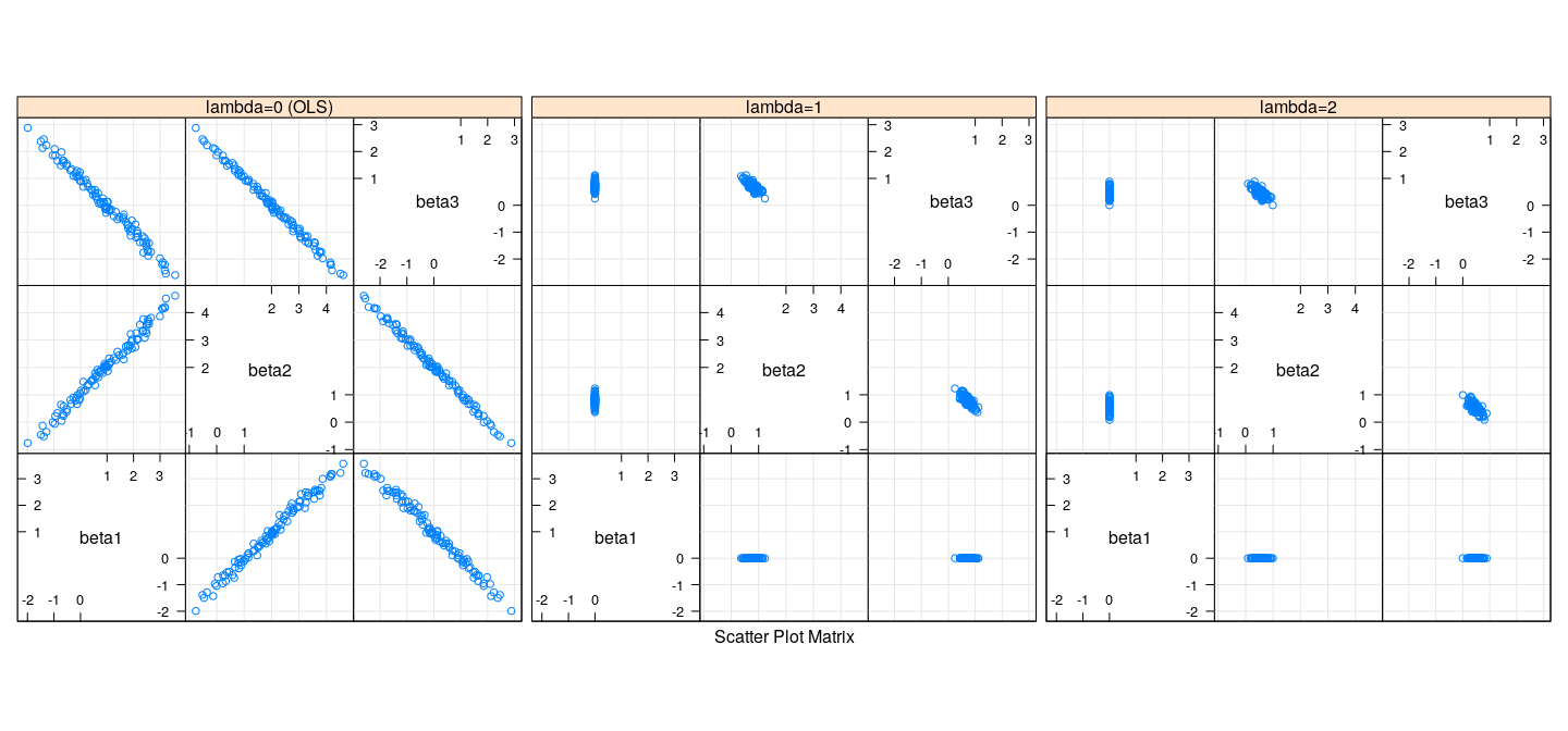
LASSO in the presence of collinearity
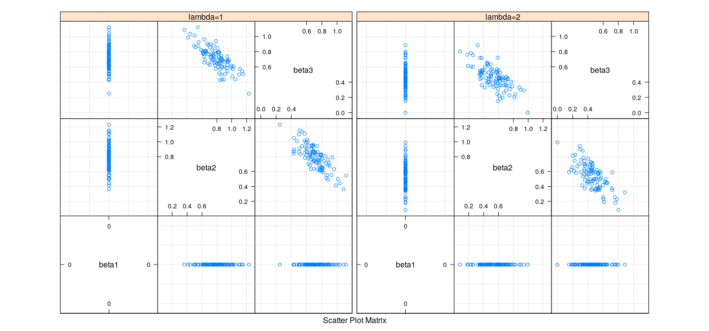
Bias and variance of LASSO
- Recall that true \(\beta = (1, 2, 0)\)
with(sim.df.lasso, rbind(tapply(beta1, which, mean),
                         tapply(beta2, which, mean),
                         tapply(beta3, which, mean)))
lambda=0 (OLS) lambda=1 lambda=2
[1,] 0.972813560 0.0000000 0.0000000
[2,] 2.008541811 0.7920059 0.5423446
[3,] -0.002656804 0.7109653 0.4587019with(sim.df.lasso, rbind(tapply(beta1, which, sd),
tapply(beta2, which, sd),
tapply(beta3, which, sd))) lambda=0 (OLS) lambda=1 lambda=2
[1,] 1.282199 0.0000000 0.0000000
[2,] 1.274482 0.1630202 0.1698728
[3,] 1.281313 0.1495002 0.1506298Coefficients as a function of \(\lambda\) : LASSO
fm.lasso <- with(d3, glmnet(cbind(x1, x2, x3), y, alpha = 1))
plot(fm.lasso, xvar = "norm", label = TRUE)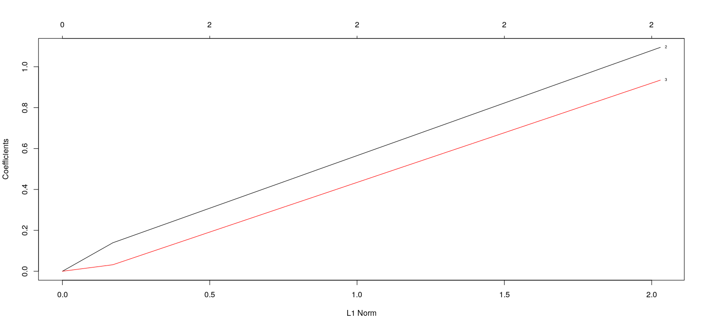
Coefficients as a function of \(\lambda\) : LASSO
fm.lasso <- with(d3, glmnet(cbind(x1, x2, x3), y, alpha = 1))
plot(fm.lasso, xvar = "dev", label = TRUE)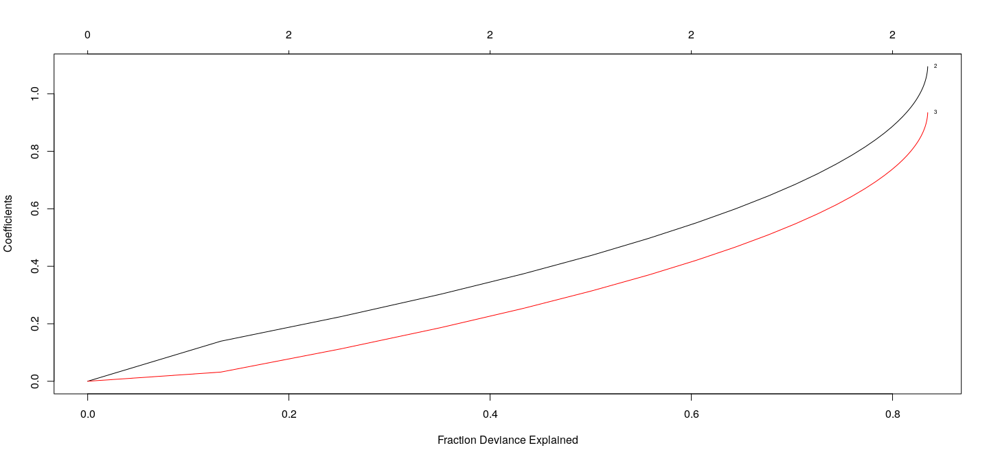
Coefficients as a function of \(\lambda\) : Ridge
fm.ridge <- with(d3, glmnet(cbind(x1, x2, x3), y, alpha = 0))
plot(fm.ridge, xvar = "norm", label = TRUE)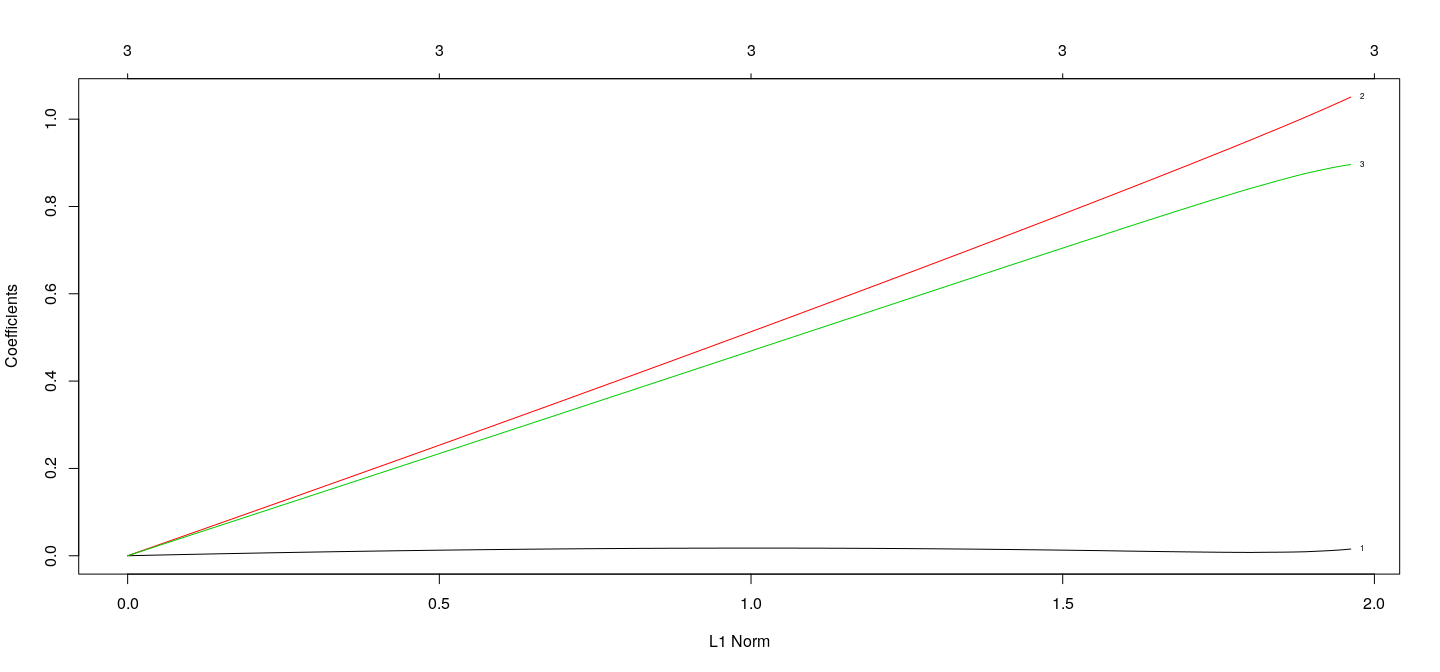
Coefficients as a function of \(\lambda\) : Ridge
fm.ridge <- with(d3, glmnet(cbind(x1, x2, x3), y, alpha = 0))
plot(fm.ridge, xvar = "dev", label = TRUE)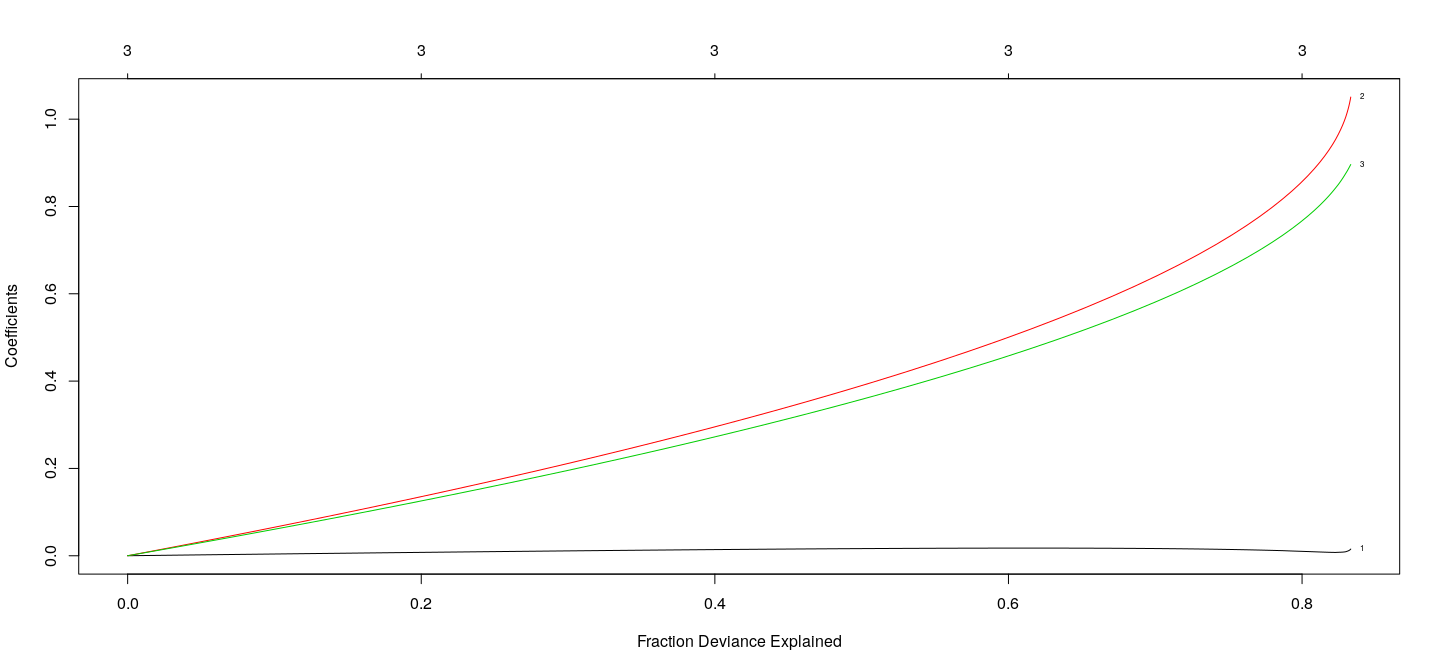
Example: Salary of hitters in Major League Baseball (1987)
'data.frame':   322 obs. of  20 variables:
 $ AtBat    : int  293 315 479 496 321 594 185 298 323 401 ...
 $ Hits     : int  66 81 130 141 87 169 37 73 81 92 ...
 $ HmRun    : int  1 7 18 20 10 4 1 0 6 17 ...
 $ Runs     : int  30 24 66 65 39 74 23 24 26 49 ...
 $ RBI      : int  29 38 72 78 42 51 8 24 32 66 ...
 $ Walks    : int  14 39 76 37 30 35 21 7 8 65 ...
 $ Years    : int  1 14 3 11 2 11 2 3 2 13 ...
 $ CAtBat   : int  293 3449 1624 5628 396 4408 214 509 341 5206 ...
 $ CHits    : int  66 835 457 1575 101 1133 42 108 86 1332 ...
 $ CHmRun   : int  1 69 63 225 12 19 1 0 6 253 ...
 $ CRuns    : int  30 321 224 828 48 501 30 41 32 784 ...
 $ CRBI     : int  29 414 266 838 46 336 9 37 34 890 ...
 $ CWalks   : int  14 375 263 354 33 194 24 12 8 866 ...
 $ League   : Factor w/ 2 levels "A","N": 1 2 1 2 2 1 2 1 2 1 ...
 $ Division : Factor w/ 2 levels "E","W": 1 2 2 1 1 2 1 2 2 1 ...
 $ PutOuts  : int  446 632 880 200 805 282 76 121 143 0 ...
 $ Assists  : int  33 43 82 11 40 421 127 283 290 0 ...
 $ Errors   : int  20 10 14 3 4 25 7 9 19 0 ...
 $ Salary   : num  NA 475 480 500 91.5 750 70 100 75 1100 ...
 $ NewLeague: Factor w/ 2 levels "A","N": 1 2 1 2 2 1 1 1 2 1 ...
Example: Salary of hitters in Major League Baseball (1987)
[1] 263 20y <- Hitters$Salary
X <- model.matrix( ~ . - Salary - 1, Hitters) # converts factors into dummy variables
fm.lasso <- glmnet(X, y, alpha = 1)
fm.ridge <- glmnet(X, y, alpha = 0)
Example: Salary of hitters in Major League Baseball (1987)
## top axis labels indicate number of nonzero coefficients
plot(fm.lasso, xvar = "lambda", label = TRUE)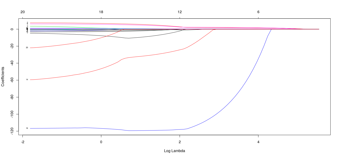
Example: Salary of hitters in Major League Baseball (1987)
## top axis labels indicate number of nonzero coefficients
plot(fm.lasso, xvar = "dev", label = TRUE)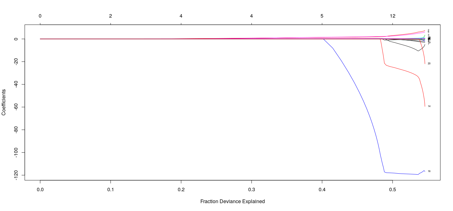
Example: Salary of hitters in Major League Baseball (1987)
## top axis labels indicate number of nonzero coefficients (not useful for Ridge)
plot(fm.ridge, xvar = "lambda", label = TRUE)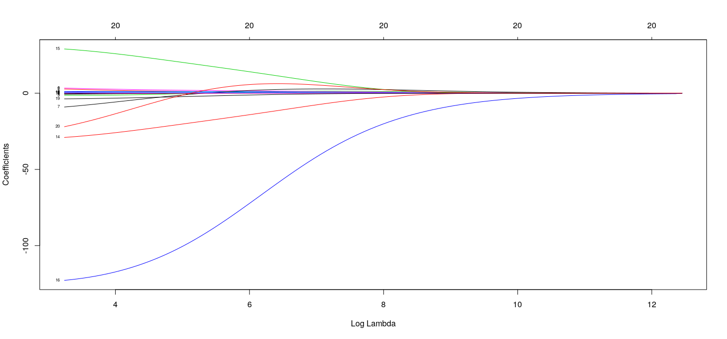
Choosing \(\lambda\)
Usual model selection criteria can be used (AIC, BIC, etc.)
Using cross-validation is more common
Note that there is no closed form expression for \(e_{i(-i)}\) in general
Leave-one-out (\(n\)-fold) cross-validation is computationally intensive for large data sets
The
cv.glmnet()function performs \(k\)-fold cross-validation (\(k=10\) by default)Divides dataset randomly into \(k\) (roughly) equal parts
Predicts on each part using model fit with remaining \((k-1)\) parts
Computes overall prediction error
Choosing \(\lambda\)
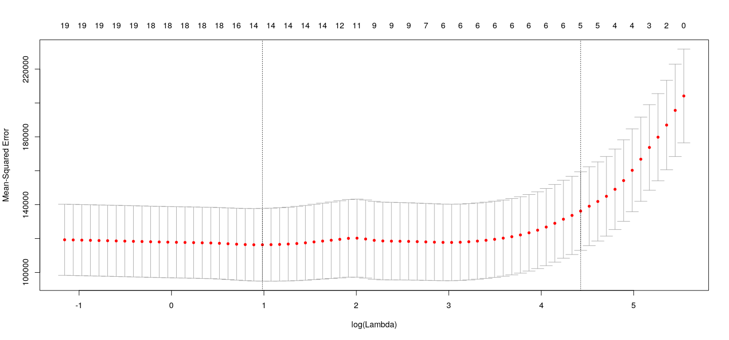
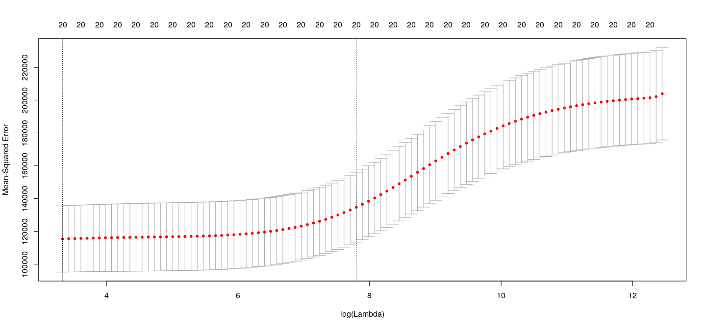
Choosing \(\lambda\)
The two lines on the plot correspond to
\(\lambda\) that minimizes cross-validation error
largest value of \(\lambda\) such that error is within 1 standard error of the minimum
lambda.min lambda.1se
  2.674375  83.593378
Choosing \(\lambda\)
s.cv <- c(lambda.min = cv.lasso$lambda.min, lambda.1se = cv.lasso$lambda.1se)
round(coef(cv.lasso, s = s.cv), 3) # corresponding coefficients
21 x 2 sparse Matrix of class "dgCMatrix"
1 2
(Intercept) 155.817 167.912
AtBat -1.547 .
Hits 5.661 1.293
HmRun . .
Runs . .
RBI . .
Walks 4.730 1.398
Years -9.596 .
CAtBat . .
CHits . .
CHmRun 0.511 .
CRuns 0.659 0.142
CRBI 0.393 0.322
CWalks -0.529 .
LeagueA -32.065 .
LeagueN 0.000 .
DivisionW -119.299 .
PutOuts 0.272 0.047
Assists 0.173 .
Errors -2.059 .
NewLeagueN . . Choosing \(\lambda\)
How well does LASSO work for variable selection?
We repeat our earlier simulation example
Let us look at number of variables selected when none are related to the response
## Replicate this experiment
num.nonzero.coefs <-
    replicate(100,
    {
        d <- matrix(rnorm(100 * 21), 100, 21)
        cv.lasso <- cv.glmnet(x = d[,-1], y = d[,1])
        lambda.cv <- cv.lasso$lambda.1se
        sum(coef(cv.lasso, s = lambda.cv)[-1] != 0) # exclude intercept
    })
table(num.nonzero.coefs)
num.nonzero.coefs
0 2
99 1
- So Type-I error probability is much lower for LASSO compared to stepwise regression
How well does LASSO work for variable selection?
- How about power to detect effects that are present? Choose \(\beta_1, \beta_2 \sim U(-1, 1)\), other \(\beta_j = 0\)
coefs <- replicate(100,
{
    X <- matrix(rnorm(100 * 20), 100, 20)
    y <- X[,1:2] %*% runif(2, -1, 1) + rnorm(100)
    cv.lasso <- cv.glmnet(X, y)
    lambda.cv <- cv.lasso$lambda.1se
    coef(cv.lasso, s = lambda.cv)[-1] # exclude intercept
})
coefs[coefs == 0] <- NA
levelplot(t(coefs), col.regions = heat.colors, xlab = "Replication number", ylab = "Coefficient number")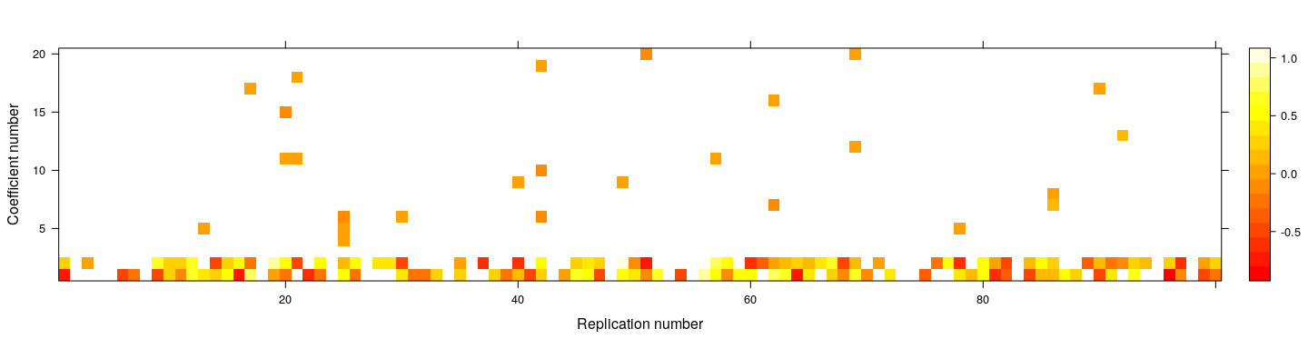
Why does LASSO lead to exact 0 coefficients?
- Alternative formulation of Ridge regression: consider problem of minimizing
\[ \sum_{i=1}^n (y_i - \mathbf{x}_i^T \beta)^2 \quad \text{subject to} \quad \lVert \beta \rVert^2 = \sum \beta_j^2 \leq t \]
Claim: The solution \(\hat{\beta}\) is the usual Ridge estimate for some \(\lambda\)
Case 1 : \(\lVert \hat{\beta}_{OLS} \rVert^2 \leq t \implies \hat{\beta} = \hat{\beta}_{OLS}, \lambda = 0\)
Case 2 : \(\lVert \hat{\beta}_{OLS} \rVert^2 > t\)
- Then must have \(\lVert \hat{\beta} \rVert^2 = t\) (otherwise can move closer to \(\hat{\beta}_{OLS}\))
- The Lagrangian is \(\lVert \mathbf{y} - \mathbf{X} \beta \rVert^2 + \lambda \lVert \hat{\beta} \rVert^2 - \lambda t\)
- This is the same optimization problem as before
- \(\lambda\) is defined implicitly as a function of \(t\), to ensure \(\lVert \hat{\beta} \rVert^2 = t\)
The LASSO problem can be similarly formulated as: minimize \(\lVert \mathbf{y} - \mathbf{X} \beta \rVert^2\) subject to \(\sum \lvert \beta_j \rvert \leq t\)
This interpretation gives a useful geometric justification for the variable selection behaviour of LASSO
Comparative geometry of Ridge and LASSO optimization
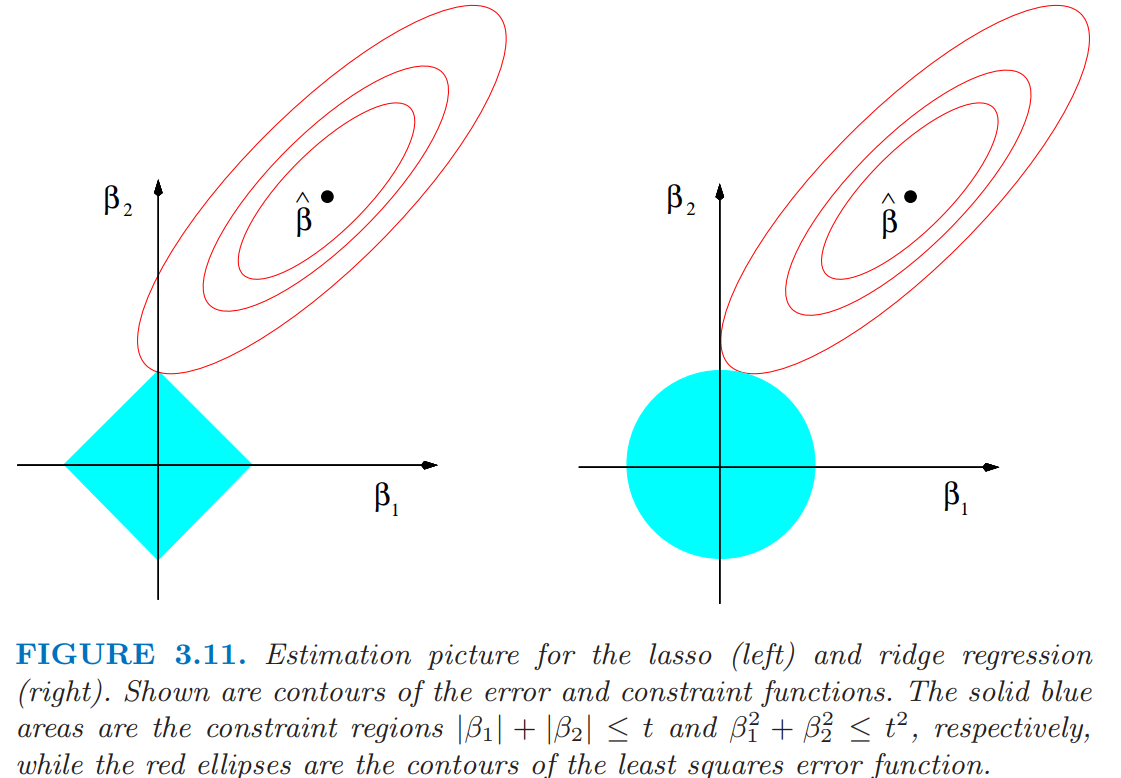
(From Elements of Statistical Learning, page 71)