Regression Techniques
Deepayan Sarkar
Regression
Most of you should be familiar with Linear Regression / Least Squares
- What is the purpose?
- What are the model assumptions?
Are there any other kinds of regression?
Course: Regression Techniques
- This course is not about linear regression!
We will
Try to refine what we understand by the term “regression” (linear regression is only a special case)
Learn alternative approaches to solve the “regression” problem
Learn how to identify and address modeling errors
Most techniques we will learn require non-trivial programming
We will learn and use the R language for computation
Room 11 (ground floor) is a computer lab (usually locked, but security guards at the main gate will open it when you ask them)
There are two more (smaller) computer labs in teh ground floor of the Faculty Building
You can use your own laptops as well
Evaluation scheme
Midterm examination: 30%
Final examination: 50%
Assignments / Projects: 20%
What is Regression?
Consider bivariate data \((X, Y)\) with some distribution
Interested in “predicting” \(Y\) for a fixed value of \(X=x\)
In probability terms, want the conditional distribution of \[Y | X = x\]
- In general
- \(Y\) could be numeric or categorical
- \(X\) could also be numeric or categorical
The “Regression Problem”: when \(Y\) is numeric
The “Classification Problem”: when \(Y\) is categorical
A more modern approach is to view both as special cases of the “Learning Problem”
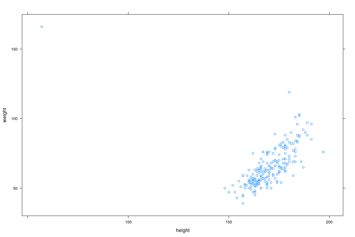
Example: Height and Weight Data
   sex weight height repwt repht
1    M     77    182    77   180
2    F     58    161    51   159
3    F     53    161    54   158
4    M     68    177    70   175
5    F     59    157    59   155
6    M     76    170    76   165
7    M     76    167    77   165
8    M     69    186    73   180
9    M     71    178    71   175
10   M     65    171    64   170
11   M     70    175    75   174
12   F    166     57    56   163
13   F     51    161    52   158
14   F     64    168    64   165
15   F     52    163    57   160
16   F     65    166    66   165
17   M     92    187   101   185
18   F     62    168    62   165
19   M     76    197    75   200
20   F     61    175    61   171
Interested in predicting weight distribution as a function of height
How should we proceed?
Example: Height and Weight Data
Example: Height and Weight Data
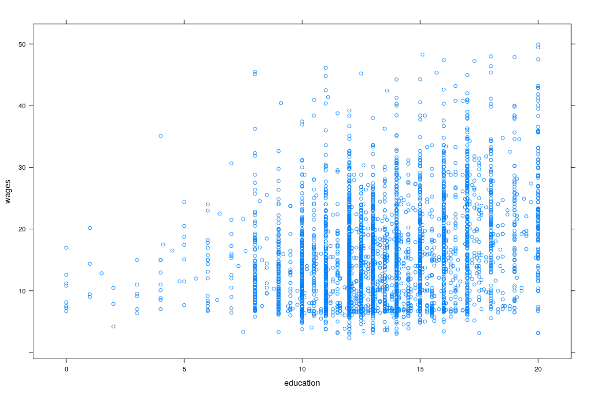
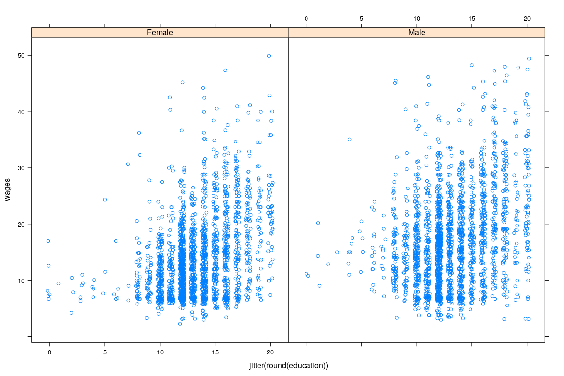
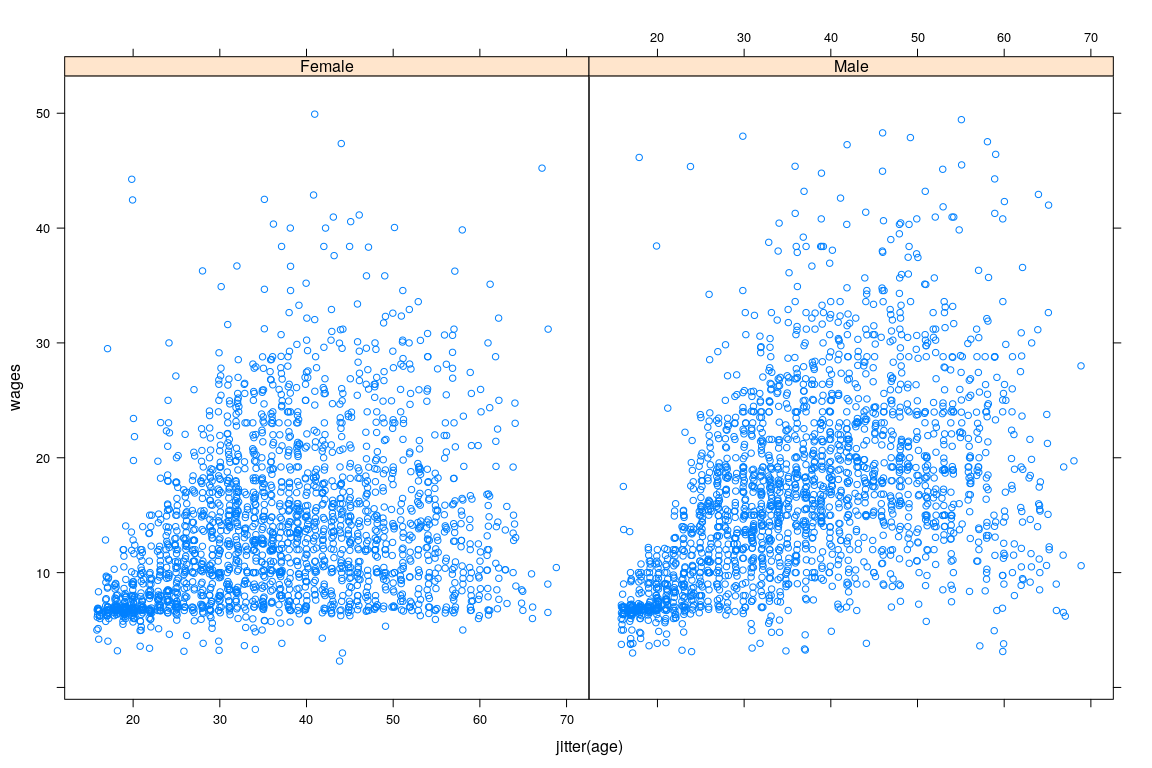
Example: Survey of Labour and Income Dynamics
'data.frame':   7425 obs. of  5 variables:
 $ wages    : num  10.6 11 NA 17.8 NA ...
 $ education: num  15 13.2 16 14 8 16 12 14.5 15 10 ...
 $ age      : int  40 19 49 46 71 50 70 42 31 56 ...
 $ sex      : Factor w/ 2 levels "Female","Male": 2 2 2 2 2 1 1 1 2 1 ...
$ language : Factor w/ 3 levels "English","French",..: 1 1 3 3 1 1 1 1 1 1 ... wages education age sex language
1 10.56 15.0 40 Male English
2 11.00 13.2 19 Male English
3 NA 16.0 49 Male Other
4 17.76 14.0 46 Male Other
5 NA 8.0 71 Male English
6 14.00 16.0 50 Female English
7 NA 12.0 70 Female English
8 NA 14.5 42 Female English
9 8.20 15.0 31 Male English
10 NA 10.0 56 Female English- Interested in predicting wage
Example: Survey of Labour and Income Dynamics
Example: Survey of Labour and Income Dynamics
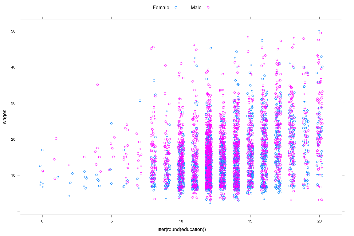
Example: Survey of Labour and Income Dynamics
Example: Survey of Labour and Income Dynamics
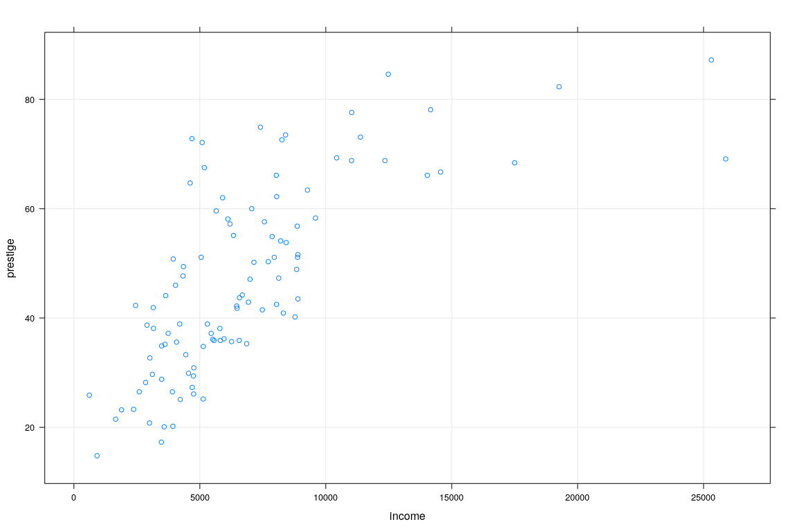
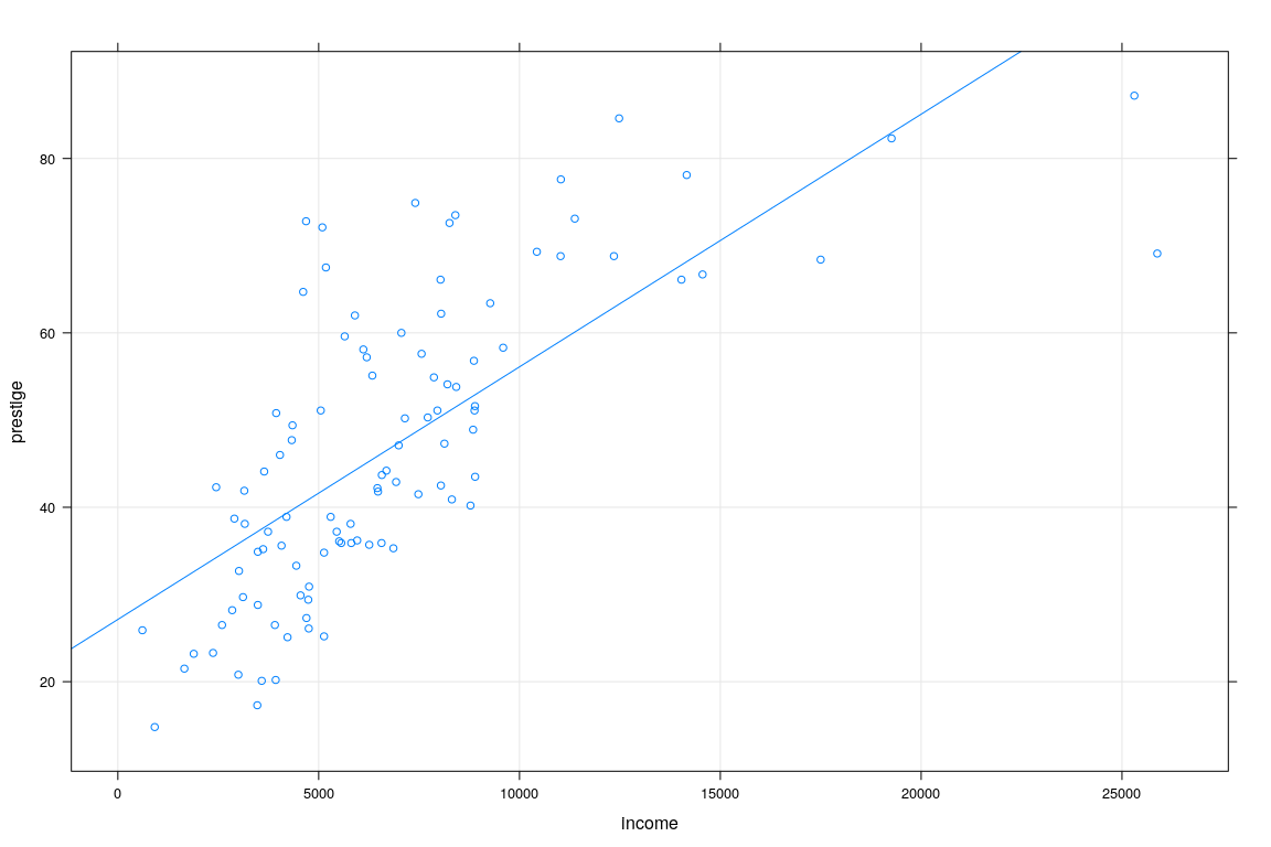
Example: Prestige vs Average income (Canada, 1971)
                       education income women prestige census type
gov.administrators         13.11  12351 11.16     68.8   1113 prof
general.managers           12.26  25879  4.02     69.1   1130 prof
accountants                12.77   9271 15.70     63.4   1171 prof
purchasing.officers        11.42   8865  9.11     56.8   1175 prof
chemists                   14.62   8403 11.68     73.5   2111 prof
physicists                 15.64  11030  5.13     77.6   2113 prof
biologists                 15.09   8258 25.65     72.6   2133 prof
architects                 15.44  14163  2.69     78.1   2141 prof
civil.engineers            14.52  11377  1.03     73.1   2143 prof
mining.engineers           14.64  11023  0.94     68.8   2153 prof
surveyors                  12.39   5902  1.91     62.0   2161 prof
draughtsmen                12.30   7059  7.83     60.0   2163 prof
computer.programers        13.83   8425 15.33     53.8   2183 prof
economists                 14.44   8049 57.31     62.2   2311 prof
psychologists              14.36   7405 48.28     74.9   2315 prof
social.workers             14.21   6336 54.77     55.1   2331 prof
lawyers                    15.77  19263  5.13     82.3   2343 prof
librarians                 14.15   6112 77.10     58.1   2351 prof
vocational.counsellors     15.22   9593 34.89     58.3   2391 prof
ministers                  14.50   4686  4.14     72.8   2511 prof
Example: Prestige vs Average income (Canada, 1971)
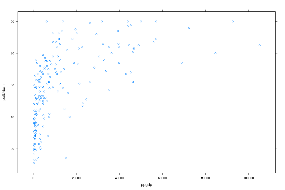
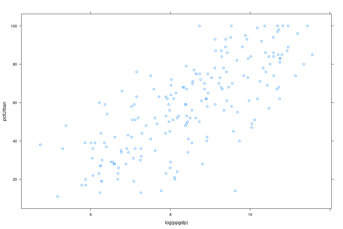
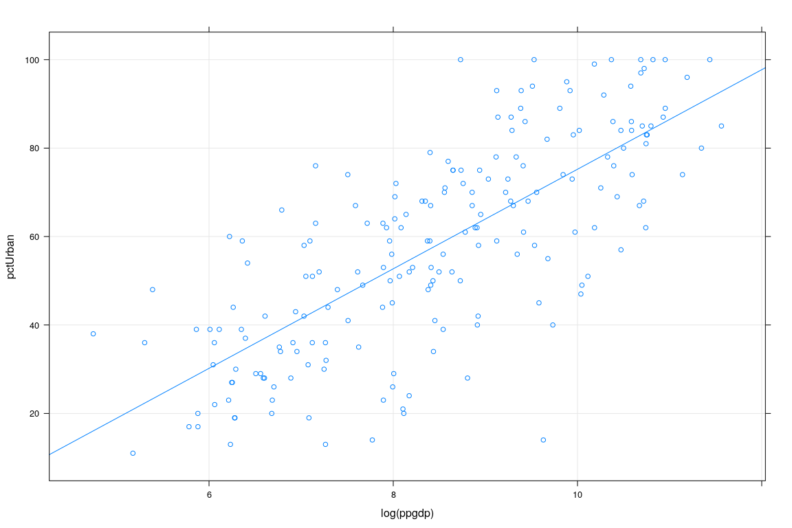
Example: UN National Statistics
                   region  group fertility   ppgdp lifeExpF pctUrban infantMortality
Afghanistan          Asia  other     5.968   499.0    49.49       23       124.53500
Albania            Europe  other     1.525  3677.2    80.40       53        16.56100
Algeria            Africa africa     2.142  4473.0    75.00       67        21.45800
American Samoa       <NA>   <NA>        NA      NA       NA       NA        11.29389
Angola             Africa africa     5.135  4321.9    53.17       59        96.19100
Anguilla        Caribbean  other     2.000 13750.1    81.10      100              NA
Argentina      Latin Amer  other     2.172  9162.1    79.89       93        12.33700
Armenia              Asia  other     1.735  3030.7    77.33       64        24.27200
Aruba           Caribbean  other     1.671 22851.5    77.75       47        14.68700
Australia         Oceania   oecd     1.949 57118.9    84.27       89         4.45500
Austria            Europe   oecd     1.346 45158.8    83.55       68         3.71300
Azerbaijan           Asia  other     2.148  5637.6    73.66       52        37.56600
Bahamas         Caribbean  other     1.877 22461.6    78.85       84        14.13500
Bahrain              Asia  other     2.430 18184.1    76.06       89         6.66300
Bangladesh           Asia  other     2.157   670.4    70.23       29        41.78600
Barbados        Caribbean  other     1.575 14497.3    80.26       45        12.28400
Belarus            Europe  other     1.479  5702.0    76.37       75         6.49400
Belgium            Europe   oecd     1.835 43814.8    82.81       97         3.73900
Belize         Latin Amer  other     2.679  4495.8    77.81       53        16.20000
Benin Africa africa 5.078 741.1 58.66 42 76.67400- Interested in predicting
pctUrbanusingppgdp
Example: UN Data
Example: UN Data
Review of Linear Regression
Interested in “predicting” \(Y\) for a fixed value of \(X=x\)
In probability terms, want the conditional distribution of \[Y | X = x\]
Important special case: linear regression
Appropriate under certain model assumptions
Essential component in more general procedures
You will learn theory in Linear Model course
We will review basics
Conditional distribution
\[Y | X = x\]
In general, the conditional distribution can be anything
If \((X, Y)\) is jointly Normal, then \[Y | X = x \sim N(\alpha + \beta x, \sigma^2)\]
for some \(\alpha, \beta, \sigma^2\)This is the motivation for Linear Regression
Correlation: Measuring linear dependence
Suppose \(E(X) = \mu_X\) and \(E(Y) = \mu_Y\)
The covariance of \(X\) and \(Y\) is defined by
\[ Cov\left(X,Y\right) = E\bigl( (X-\mu_X ) ( Y-\mu_Y) \bigr) = E(XY) - \mu_X \, \mu_Y \]
The correlation coefficient \(\rho \left( X,Y \right)\) of \(X\) and \(Y\) is defined by
\[ \rho (X,Y)=\frac{Cov\left( X,Y\right) }{\sqrt{Var \left( X\right) Var\left( Y\right) }} \]
Properties of Correlation Coefficient
\(-1 \leq \rho \leq 1\)
\(\rho = -1\): perfect decreasing linear relation
\(\rho = 1\): perfect increasing linear relation
\(\rho = 0\): no linear relation
Sample Correlation
Sample analog of correlation
\[ r(X,Y)=\frac{\sum_i (x_i - \bar x) (y_i - \bar y)} {\sqrt{ \sum_i (x_i - \bar x)^2 \sum_i (y_i - \bar y)^2 }} \]
Closely related with regression
Correlation between height and weight (
Davisdata): 0.19Correlation between reported height and weight (
Davisdata): 0.762Correlations in labour dynamics data
| wages | education | age | |
|---|---|---|---|
| wages | 1.000 | 0.307 | 0.361 |
| education | 0.307 | 1.000 | -0.298 |
| age | 0.361 | -0.298 | 1.000 |
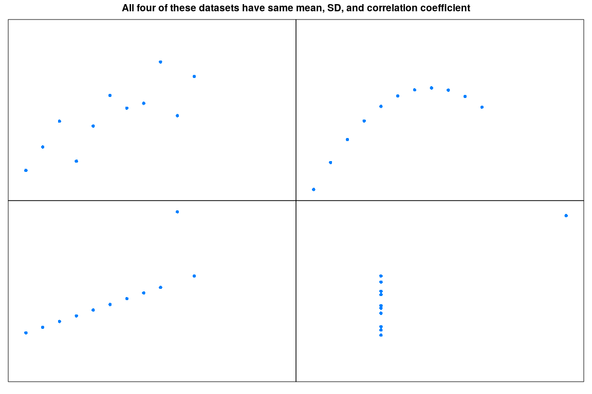
Warning! Correlation only measures linear relation!
(Multiple) Linear Regression
In general form, the regression model assumes
\[ E(Y | X_1 = x_1, X_2 = x_2, \dotsc, X_p = x_p) = \beta_0 + \sum_{j=1}^p \beta_j x_j \] \[ Var(Y | X_1 = x_1, X_2 = x_2, \dotsc, X_p = x_p) = \sigma^2 \]
where
\(\beta_0, \beta_1, \dotsc, \beta_p, \sigma^2 > 0\) are unknown parameters
\(X_1, X_2, \dotsc, X_p\) are (conditionally) fixed covariates
\(X_1, X_2, \dotsc, X_p\) may be derived from a smaller set of predictors, e.g.,
- \(X_2 = Z_1\) (linear term for \(Z_1\))
- \(X_3 = Z_2\) (linear term for \(Z_2\))
- \(X_4 = Z_1^2\) (quadratic term for \(Z_1\))
- \(X_5 = Z_2^2\) (quadratic term for \(Z_2\))
- \(X_6 = Z_1 Z_2\) (interaction term)
(Multiple) Linear Regression
In vector notation (incorporating intercept term in \(\mathbf{X}\))
\[ E(Y | \mathbf{X} = \mathbf{x}) = \mathbf{x}^T \mathbf{\beta} \] \[ Var(Y | \mathbf{X} = \mathbf{x}) = \sigma^2 \]
Alternatively
\[ Y = \mathbf{x}^T \mathbf{\beta} + \varepsilon \text{ where }\] \[ E(\varepsilon) = 0, Var(\varepsilon) = \sigma^2\]
Sample version: \(n\) independent observations from this model
- For \(i\)th sample point, let
- \(Y_{i}=\) response
- \(\mathbf{x}_{i}=\) \(p\)-dimensional vector of predictors
We assume that
\[ Y_{i}=\mathbf{x}_{i}^T\mathbf{\beta} + \varepsilon_{i}, \]
where \(\varepsilon_i\) are independent and
\[ E(\varepsilon_{i}) = 0, Var(\varepsilon_i) = \sigma^2 \]
In matrix notation
\[ \mathbf{Y}= \mathbf{X} \mathbf{\beta} + \mathbf{\varepsilon} \]
where \[ \mathbf{Y}=\left( \begin{array}{c} Y_{1} \\ \vdots \\ Y_{n} \end{array} \right),\, \mathbf{X=}\left( \begin{array}{c} \mathbf{x}_{1}^T \\ \vdots \\ \mathbf{x}_{n}^T \end{array} \right),\, \mathbf{\varepsilon} = \left( \begin{array}{c} \varepsilon_{1} \\ \vdots \\ \varepsilon_{n} \end{array} \right) \]
\(\mathbf{Y}\) and \(\mathbf{\varepsilon}\) are \(n\times1\)
\(\mathbf{X}\) is \(n\times p\)
Columns of \(\mathbf{X}\) are assumed to be linearly independent (\(\text{rank}(\mathbf{X}) = p\))
\(\mathbf{\beta}_{p\times 1}\) and \(\sigma^2 > 0\) are unknown parameters
Problem: How to estimate \(\mathbf{\beta}\) and \(\sigma^2\)
- Least squares approach: minimize sum of squared errors \[ \widehat{\mathbf{\beta}} = \arg\min_{\mathbf{\beta}} q(\mathbf{\beta}) \] where \[ q(\mathbf{\beta}) = \sum (Y_{i} - \mathbf{x}_{i}^T \mathbf{\beta})^{2} = (\mathbf{Y} - \mathbf{X} \mathbf{\beta})^T (\mathbf{Y} - \mathbf{X}\mathbf{\beta}) \]
Problem: How to estimate \(\mathbf{\beta}\) and \(\sigma^2\)
- Set gradient with respect to \(\mathbf{\beta}\) to \(\mathbf{0}\).
\[ \nabla q(\mathbf{\beta}) = 2 \mathbf{X}^T (\mathbf{Y-X\beta}) = 2 (\mathbf{X}^T \mathbf{Y-X}^T \mathbf{X \beta}) = \mathbf{0} \]
- This leads to Normal Equations:
\[ \mathbf{X}^T \mathbf{X \beta} = \mathbf{X}^T \mathbf{Y} \]
- Estimate of \(\mathbf{\beta}\) assuming that \(\mathbf{X}^T \mathbf{X}\) has full rank (OLS estimator):
\[ \widehat{\mathbf{\beta }} = ( \mathbf{X}^T \mathbf{X})^{-1} \mathbf{X}^T \mathbf{Y} \]
The OLS estimator in practice
fm1 <- lm(weight ~ height, data = Davis)
xyplot(weight ~ height, data = Davis, grid = TRUE, type = c("p", "r"))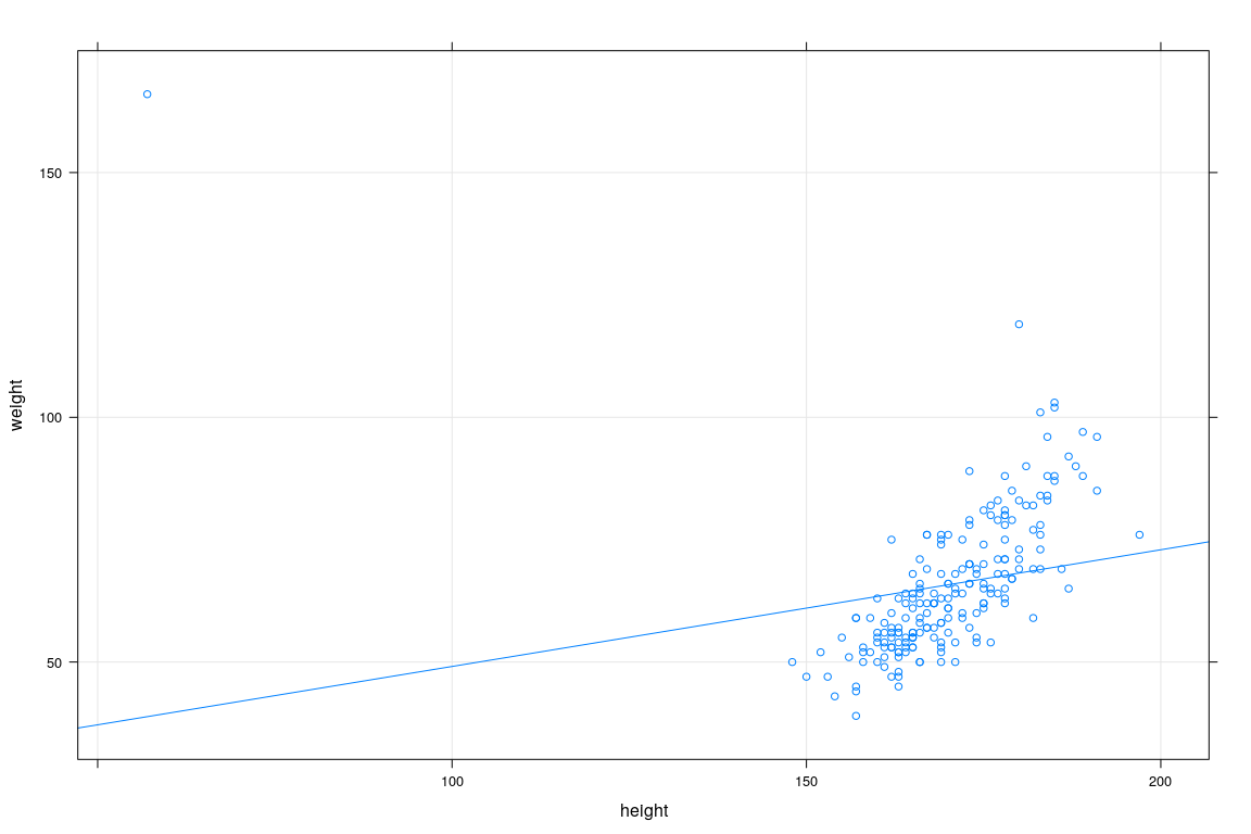
The OLS estimator in practice
fm1 <- lm(repwt ~ repht, data = Davis)
xyplot(repwt ~ repht, data = Davis, grid = TRUE, type = c("p", "r"))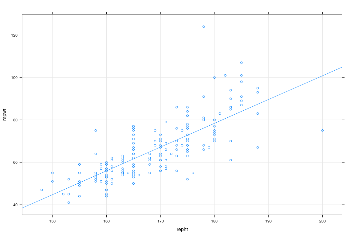
The OLS estimator in practice
The OLS estimator in practice
Alternative approach: maximum likelihood
Less arbitrary, but needs model assumption: Multivariate Normality
To indicate that \(\mathbf{Y}\) follows \(n\)-dimensional Multivariate Normal Distribution with mean vector \(\mu\) and covariance matrix \(\Sigma\), we write
\[ \mathbf{Y} \sim N_{n}\left(\mathbf{\mu}, \Sigma \right) \]
When \(\Sigma\) has full rank (positive definite), \(\mathbf{Y}\) has joint density function (pdf)
\[ f\left(\mathbf{y}\right) = \left( 2\pi \right) ^{-n/2}\left\vert {\Sigma }\right\vert ^{-1/2} \exp\left\lbrace -\frac{1}{2} (\mathbf{y-\mu})^T \Sigma^{-1} (\mathbf{y-\mu}) \right\rbrace \]
Note that this function has the two worst things in matrices, the determinant and the inverse of a matrix.
Alternative approach: maximum likelihood
Fortunately, the situation is simpler for the regression model \[ \mathbf{Y} \sim N_n(\mathbf{X\beta}, \sigma^2 \mathbf{I}) \] with probability density function \[ f(\mathbf{y}) = (2\pi)^{-n/2} \left( \sigma ^{2}\right)^{-n/2} \exp\left\lbrace -\frac{1}{2\sigma^2}\left\Vert \mathbf{y-X\beta }\right\Vert ^{2} \right\rbrace \]
Therefore the likelihood for this model is \[ L\left( \mathbf{\beta}, \sigma^{2} \right) = \left( 2\pi \right) ^{-n/2}\left( \sigma ^{2}\right) ^{-n/2} \exp\left\lbrace -\frac{1}{2\sigma^2}\left\Vert \mathbf{Y-X\beta }\right\Vert^{2} \right\rbrace \]
Maximizing \(L\left( \mathbf{\beta}, \sigma^{2} \right)\) w.r.t. \(\mathbf{\beta}\) is equivalent to minimizing \(\left\Vert \mathbf{Y-X\beta }\right\Vert^{2}\)
Is this a good estimator?
To answer this, we need some more tools
Mean and Covariance of a random vector \(\mathbf{Y}\) \[ \mathbf{\mu} = \left( \begin{array}{c} \mu _{1} \\ \vdots \\ \mu _{n} \end{array} \right),\, \Sigma = \left( \begin{array}{ccc} \Sigma _{11} & \cdots & \Sigma _{1n} \\ \vdots & \ddots & \vdots \\ \Sigma _{n1} & \cdots & \Sigma _{nn} \end{array} \right) \] where \[ \mu_{i}=EY_{i}, \] and \[ \Sigma_{ij}=\begin{cases} Var( Y_{i} ) & \text{for } i=j\\ Cov( Y_{i},Y_{j} ) & \text{for } i\neq j \end{cases} \]
Properties of mean and covariance
The covariance matrix is symmetric
For any \(n\times n\) matrix \(\mathbf{A}\) and \(n\times 1\) vector \(\mathbf{b}\)
\[ E\left( \mathbf{AY+b}\right) =\mathbf{A}E(\mathbf{Y}) + \mathbf{b},\text{ } \]
\[ Cov(\mathbf{AY+b}) = \mathbf{A} Cov(\mathbf{Y}) \mathbf{A}^T \]
Variance of a linear combination
\[ 0 \leq Var(\mathbf{a}^T \mathbf{Y}) = \mathbf{a}^T Cov(\mathbf{Y}) \mathbf{a} \]
which implies that the covariance matrix is non-negative definite.
Properties of the OLS estimator \(\widehat{\mathbf{\beta}}\)
Mean: \[ E\widehat{\mathbf{\beta}} = \left( \mathbf{X}^T \mathbf{X} \right)^{-1} \mathbf{X}^T E\mathbf{Y} = \left( \mathbf{X}^T \mathbf{X} \right)^{-1} \mathbf{X}^T \mathbf{X\beta} =\mathbf{\beta} \]
Covariance: \[ Cov(\widehat{\mathbf{\beta}}) = \left( \mathbf{X}^T \mathbf{X}\right) ^{-1}\mathbf{X}^T \sigma^2\mathbf{IX}\left( \mathbf{X}^T \mathbf{X}\right)^{-1}= \sigma^2\left( \mathbf{X}^T \mathbf{X}\right)^{-1}=\sigma^2 \mathbf{M} \]
Property of Multivariate Normal:
If \(\mathbf{Y} \sim N_n(\mathbf{\mu}, \Sigma)\), then \[ \mathbf{AY+b} \sim N( \mathbf{A\mu + b}, \mathbf{A} \Sigma \mathbf{A}^T) \]
Therefore \[ \widehat{\mathbf{\beta}}\sim N_{p}\left( \mathbf{\beta} ,\sigma^{2}\mathbf{M}\right) \]
Properties of the OLS estimator \(\widehat{\mathbf{\beta}}\)
- For the normal model, the OLS is the best unbiased estimator, i.e., it has smaller variance than any other unbiased estimator.
More precisely, \(\mathbf{\ell}^T \widehat{\mathbf{\beta}}\) is the best unbiased estimator of \(\mathbf{\ell}^T \mathbf{\beta}\) for any linear combination \(\mathbf{\ell}^T \mathbf{\beta}\).
- \(E(\mathbf{\ell}^T \widehat{\mathbf{\beta}}) = \mathbf{\ell}^T \mathbf{\beta}\)
- \(Var(\mathbf{\ell}^T \widehat{\mathbf{\beta}}) = \sigma^2 \mathbf{\ell}^T \left( \mathbf{X}^T \mathbf{X}\right)^{-1} \mathbf{\ell}\)
- Note that this conditional variance depends on \(\mathbf{X}\) — does distribution of \(\mathbf{X}\) matter?
- Prediction: Put \(\mathbf{\ell} = \mathbf{x}\) for some future covariates \(\mathbf{x}\)
Even without assuming normality, the OLS estimator has smaller variance than any other linear unbiased estimator.
The OLS estimator is consistent (as long as \(\mathbf{X}\) grows reasonably), i.e., \(\widehat{\mathbf{\beta}} \to \beta\) as \(n \to \infty\).
The unbiased estimator of \(\sigma^{2}\)
We typically estimate \(\sigma ^{2}\) by \[ \widehat{\sigma }^{2}=\left\Vert \mathbf{Y-X}\widehat{\beta }\right\Vert^{2}/\left( n-p\right) \] which is called the unbiased estimator of \(\sigma ^{2}\)
Distribution of \(\widehat{\sigma }^{2}\): \[ \frac{\left( n-p\right) \widehat{\sigma }^{2}}{\sigma ^{2}}\sim \chi_{n-p}^{2} \] independently of \(\widehat{\beta}\)
Properties of \(\widehat{\sigma }^{2}\)
For the normal model \(\widehat{\sigma }^{2}\) is the best unbiased estimator.
Even without normality, \(\widehat{\sigma}^{2}\) is unbiased.
\(\widehat{\sigma }^{2}\) is consistent
The maximum likelihood estimator (MLE)
To find MLE of \(\sigma^{2}\), differentiate \(\log L(\widehat{\beta}, \sigma^{2})\) with respect to \(\sigma\)
Easy to show that this gives \[ \widehat{\sigma }_{MLE}^{2} = \frac{1}{n} \left\Vert \mathbf{Y-X}\widehat{\beta }\right\Vert^{2} \]
Note that the MLE is not unbiased, but is consistent.
In general, neither the OLS estimator nor the MLE of \(\sigma^{2}\) minimize mean squared error (MSE)
Testing
We are often interested in coefficients \(\beta_{j}\)
Note that by properties given above \[ \widehat{\beta}_{j} \sim N(\beta_j, \sigma^2 M_{jj}) \]
“Standard error” of \(\widehat{\beta}_{j}\) \[ \widehat{\sigma }_{\widehat{\beta }_{j}}=\widehat{\sigma }\sqrt{M_{jj}} \]
Testing: \(t\)-statistic
Testing the null hypothesis \(H_0 : \beta_{j} = c\) \[ t=\frac{\widehat{\beta}_{j} - c}{\widehat{\sigma}_{\widehat{\beta}_{j}}} \sim t_{n-p}. \]
- Can be generalized to:
- any linear combination of \(\beta_j\)
- more than one simultaneous restrictions (\(F\)-test)
\(t\)-tests in practice
Call:
lm(formula = weight ~ height, data = Davis)

Residuals:
    Min      1Q  Median      3Q     Max
-23.696  -9.506  -2.818   6.372 127.145

Coefficients:
            Estimate Std. Error t value Pr(>|t|)
(Intercept) 25.26623   14.95042   1.690  0.09260
height       0.23841    0.08772   2.718  0.00715

Residual standard error: 14.86 on 198 degrees of freedom
Multiple R-squared:  0.03597,   Adjusted R-squared:  0.0311
F-statistic: 7.387 on 1 and 198 DF, p-value: 0.007152\(t\)-tests - computing \(p\)-values in R
[1] 0.007150357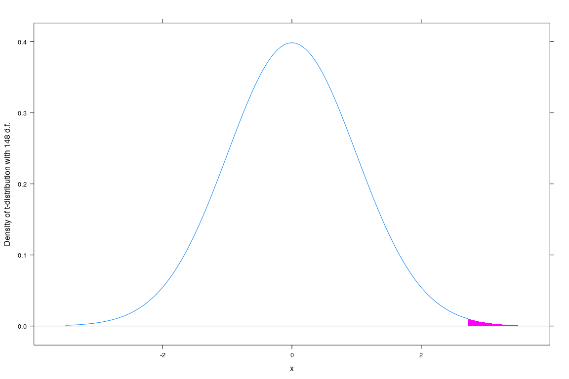
Testing: \(F\)-statistic
Loosely speaking,
Suppose we are interested in testing \(H_0\) vs \(H_1\), where \(H_0\) is a sub-model of \(H_1\)
\[ H_0 \subset H_1 \quad (H_m : \mathbf{Y} \sim N_n(\mathbf{X}_m \beta_m, \sigma^2 \mathbf{I}) ) \]
Let the sum of squared errors for the two models be \(S^2_0\) and \(S^2_1\)
\[ S^2_m = \left\Vert \mathbf{Y} - \mathbf{X}_m \widehat{\beta}_m \right\Vert^{2}, m = 0, 1 \]
Let the number of parameters (length of \(\beta\)) in the two models be \(p_0\) and \(p_1\)
Then the test statistic
\[ F = \frac{\frac{S_0^2 - S_1^2}{p_1-p_0}}{\frac{S_1^2}{n-p_1}} \text{ follows } F_{p_1-p_0, n-p_1} \text{ under } H_0 \]
(Cochran’s theorem, Linear Models course)
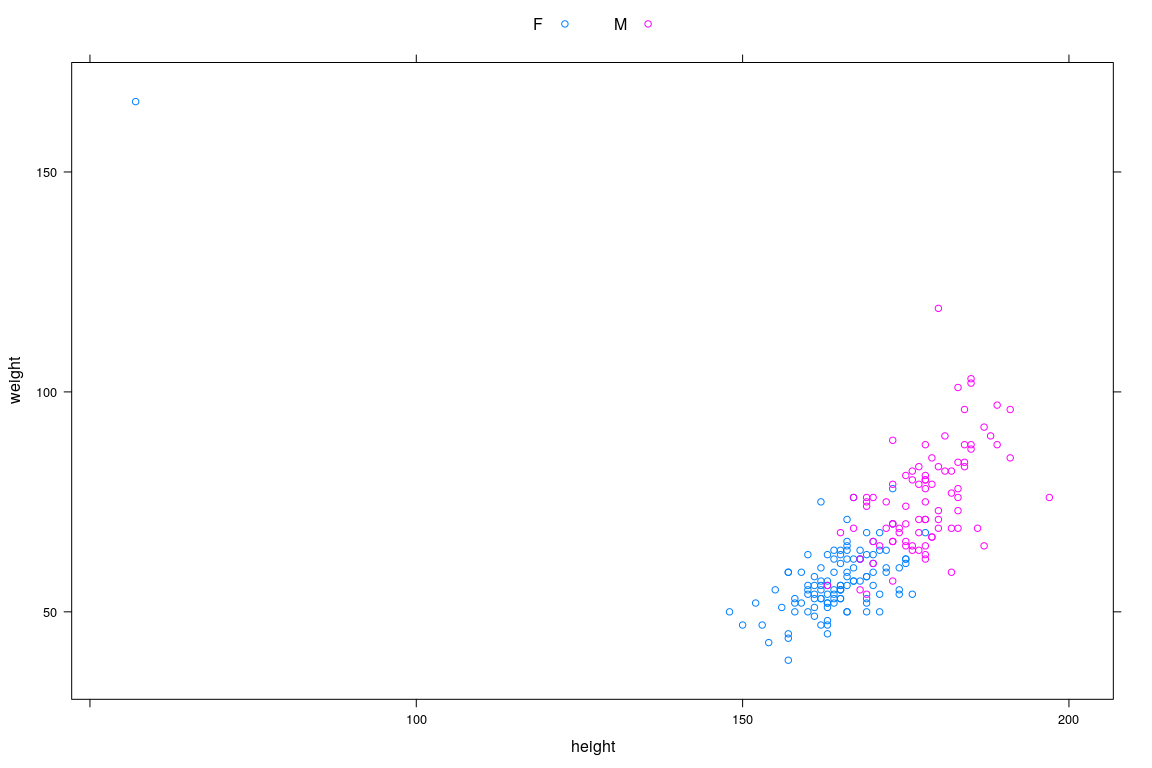
\(F\)-tests in practice
Call:
lm(formula = weight ~ height * sex, data = Davis)

Residuals:
    Min      1Q  Median      3Q     Max
-23.091  -6.331  -0.995   6.207  41.230

Coefficients:
              Estimate Std. Error t value Pr(>|t|)
(Intercept)  160.49748   13.45954  11.924  < 2e-16
height        -0.62679    0.08199  -7.644 9.17e-13
sexM        -261.82753   32.72161  -8.002 1.05e-13
height:sexM    1.62239    0.18644   8.702 1.33e-15

Residual standard error: 10.06 on 196 degrees of freedom
Multiple R-squared:  0.5626,    Adjusted R-squared:  0.556
F-statistic: 84.05 on 3 and 196 DF, p-value: < 2.2e-16\(F\)-tests in practice
Analysis of Variance Table

Model 1: weight ~ height
Model 2: weight ~ height * sex
  Res.Df   RSS Df Sum of Sq      F    Pr(>F)
1    198 43713
2    196 19831  2     23882 118.02 < 2.2e-16
Measuring Goodness of Fit: Coefficient of Determination
Consider residual sum of squared errors \[ T^{2}=\sum \left( Y_{i}-\bar{Y}\right)^{2} \] and \[ S^{2}=\sum \left( Y_{i} - \mathbf{x}_i^T \widehat{\mathbf{\beta}} \right)^{2}=\left\Vert\mathbf{Y-X}\widehat{\beta }\right\Vert ^{2} \] for intercept-only model and regression model
We can think of these as measuring the “unexplained variation” in \(\mathbf{Y}\) under these two models.
- Then the coefficient of determination \(R^{2}\) is defined by \[ R^{2}=\frac{T^{2}-S^{2}}{T^{2}} = 1 - \frac{S^{2}}{T^{2}} \] Note that \[ 0\leq R^{2}\leq 1 \]
\(R^{2}\)
\(T^{2}-S^{2}\) is the amount of variation in the intercept-only model which has been explained by including the extra predictors of the regression model and
\(R^{2}\) is the proportion of the variation left in the intercept-only model which has been explained by including the additional predictors.
Link with correlation: It can be shown that for one predictor, \[ R^2 = r^2(X, Y) \]
Adjusted \(R^2\)
Note that \[ R^{2}=\frac{\frac{T^{2}}{n}-\frac{S^{2}}{n}}{\frac{T^{2}}{n}} \]
Possible alternative: substitute unbiased estimators
Adjusted \(R^{2}\): \[ R_{a}^{2}=\frac{\frac{T^{2}}{n-1}-\frac{S^{2}}{n-p}}{\frac{T^{2}}{n-1}}=1-\frac{n-1}{n-p}( 1-R^{2}) \]
Predictive \(R^2\): Leave-One-Out Cross-validation
- Disadvantage of \(R^{2}\) and adjusted \(R^{2}\)
- Evaluates fit based on same data that is used to obtain fit
- Adding more covariates will always improve \(R^2\)
- A better procedure is based on cross-validation.
Delete the \(i\)th observation and compute \(\widehat{\mathbf{\beta}}_{(-i)}\) after excluding \(i\)th observation.
Also compute the sample mean excluding the \(i\)th observation \[ \bar{Y}_{(-i)} = \frac{1}{n-1} \sum_{j\neq i} Y_{j} \]
Do this for all \(i\).
Predictive \(R^2\): Leave-One-Out Cross-validation
- Define \[ T_{p}^{2}=\sum \left( Y_{i} - \bar{Y}_{(-i)}\right)^{2} \] and \[ S_{p}^{2}=\sum \left( Y_{i}-\mathbf{x}_{i}^T \widehat{\mathbf{\beta}}_{(-i)}\right)^{2} \]
The predictive \(R^{2}\) is defined as \[ R_{p}^{2}=\frac{T_{p}^{2}-S_{p}^{2}}{T_{p}^{2}} \]
This computes the fit to the \(i\)th observation without using that observation
Better measure of goodness of model fit than \(R^{2}\) or adjusted \(R^{2}\)
Beyond linear regression (topics of this course)
Identifying violations of linear model assumptions
- Lack of fit (linearity)
- Heteroscedasticity
- Autocorrelation in errors
- Collinearity (not a violation, but still problematic)
- Discordant outliers and influential observations
- Non-normality of errors
Possible solutions
- Nonparametric regression
- More flexible “linear” regression models (e.g., splines)
- Transformations
- Modeling heteroscedasticity
- Regularization (constrain parameters)
- Variable selection
- Robust Regression
First, get familiar with R
Many other online resources available