Diagnosing Systematic Model Violations
Deepayan Sarkar
Violation of assumptions in a linear regression model
Systematic violations
- Non-normality of errors
- Nonconstant error variance
- Lack of fit (nonlinearity)
- (Autocorrelation in errors — later)
Non-normality of errors
- Why do we care? LSE is Best Linear Unbiased Estimator under assumptions of
- linearity
- constant variance
- uncorrelated errors
Even if LSE is valid, it may not be efficient, especially with heavy tailed errors (outliers)
LSE estimates conditional mean \(f(x) = E(Y | X = x)\)
Multimodal error distribution usually indicates presense of latent covariate
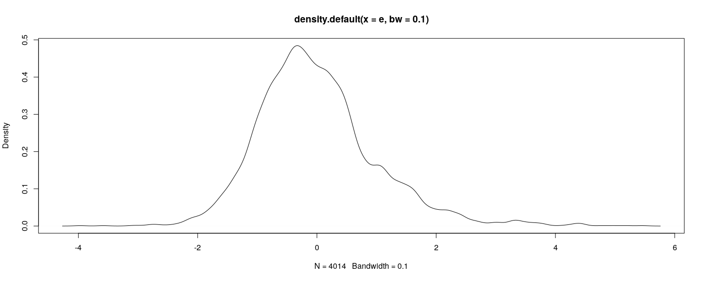
Graphical techniques
Although formal tests exist, we will focus on graphical techniques
More useful in practice because they can pinpoint nature of violation
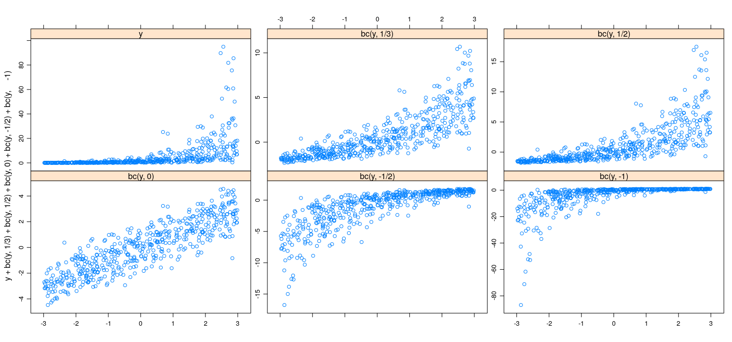
![plot of chunk unnamed-chunk-1]()
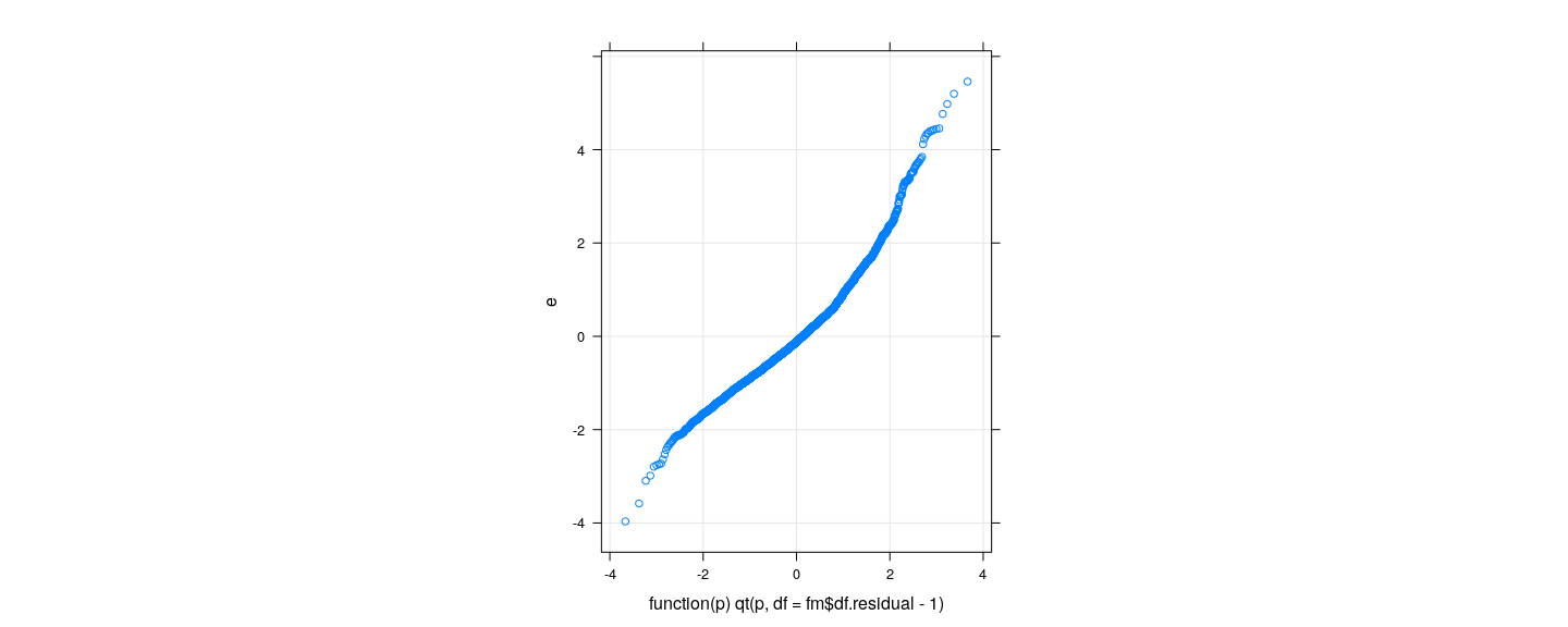
Graphical techniques
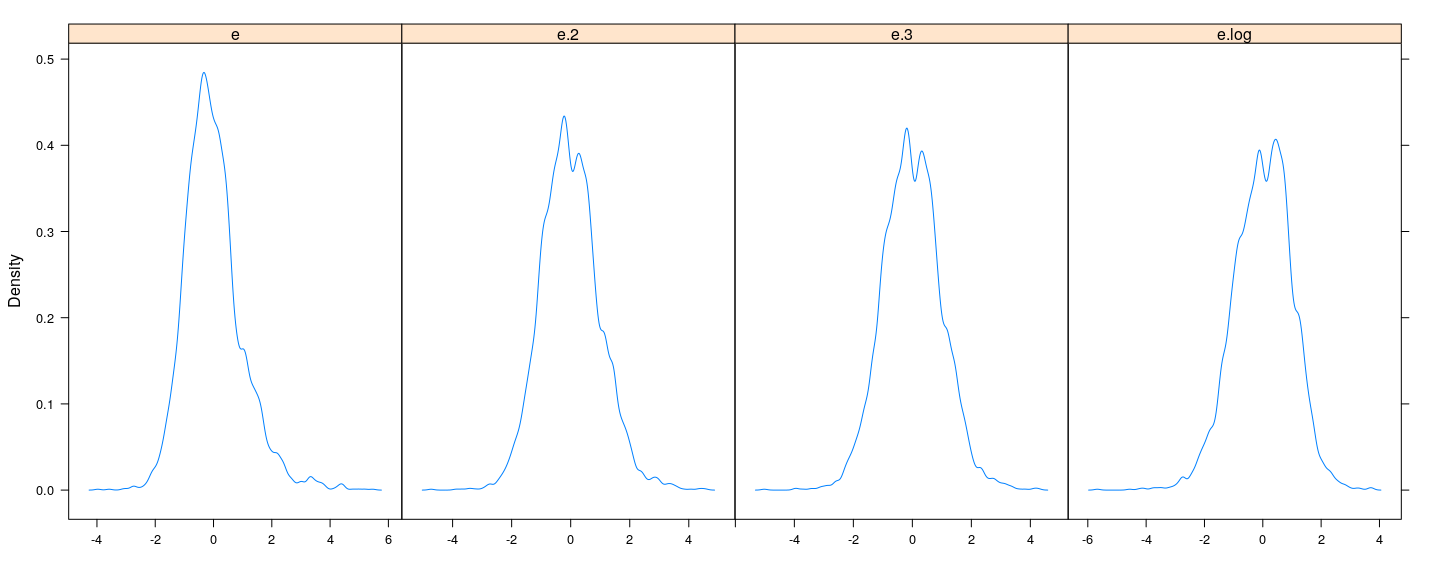
![plot of chunk unnamed-chunk-2]()
- But is there a reference to compare to?
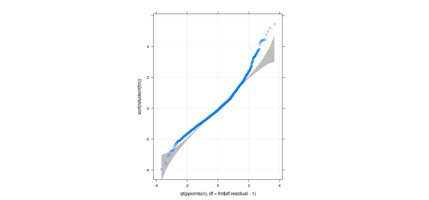
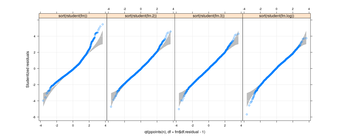
Confidence bounds for QQ-plots using Parametric Bootstrap
Confidence bounds for QQ-plots using Parametric Bootstrap
xyplot(sort(rstudent(fm)) ~ qt(ppoints(n), df = fm$df.residual - 1), grid = TRUE, aspect = "iso") +
    layer_(panel.polygon(c(x, rev(x)), c(qsim[1,], rev(qsim[2,])), col = "grey", border = NA))
![plot of chunk unnamed-chunk-4]()
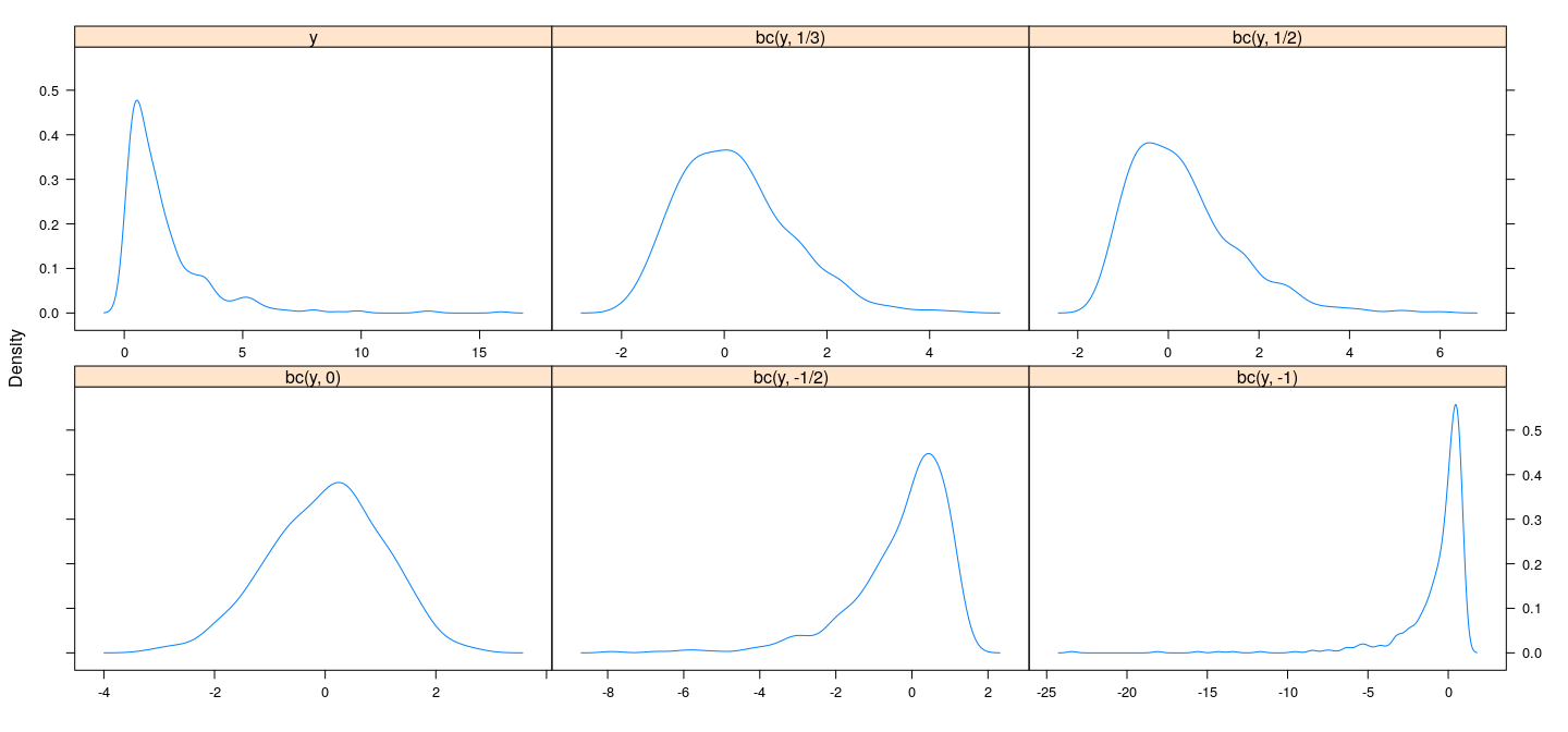
How can we address non-Normality?
Sometimes, a more general model may be appropriate (e.g., GLMs, to be studied later)
Often, transforming the response can prove useful
- E.g., variance stabilizing transformations (depending on distributions)
- \(\sqrt{y}\) for Poisson
- \(\sin^{-1} (\sqrt{y})\) for Binomial
\(\log y\) for positive-valued data (especially economic data)
Logit transform \(\log (p / (1-p))\) for proportions
More details: Kolmogorov-Smirnoff test
\[\hat{F}_n(x) = \frac{1}{n} \sum_i \mathbf{1} \{ X_i \leq x \}\]
\[T(X_1, \dotsc, X_n) = \sup_{x \in \mathbb{R}} \lvert \hat{F}_n(x) - F_0(x) \rvert\]
- Note that
- null distribution of \(T\) does not depend on \(F_0\) (use \(U_i = F_0(X_i) \sim \text{ i.i.d. } U(0, 1)\) instead)
- Intuitively, large value of \(T\) indicates departure from null, so reject when \(T\) is large
- \(p\)-value can be approximated using simulation
- Can also be estimated conservatively using the DKW inequality
More details: Shapiro-Wilk test
Null hypothesis: \(X_1, \dotsc, X_n \sim \text{ i.i.d. } N(\mu, \sigma^2)\) for some \(\mu, \sigma^2\)
Test statistic
\[W = \frac{ (\sum_i a_i X_{(i)})^2 }{\sum_i (X_i - \bar{X})^2}\]
\[\mathbf{a} = \frac{\mathbf{m}^T \mathbf{V}}{\sqrt{\mathbf{m}^T \mathbf{V}^{-1} \mathbf{V}^{-1} \mathbf{m}} }\]
with \(\mathbf{m}\) and \(\mathbf{V}\) the mean vector and variance-covariance matrix of \((Z_{(1)}, \dotsc, Z_{(n)})^T\), where \(Z_1, \dotsc, Z_n \sim \text{ i.i.d. } N(0, 1)\)
The motivation (and implementation) for this test is slightly complicated, but the basic idea is that \(\sum_i a_i X_{(i)}\) estimates the slope of the Normal Q-Q plot (which is an estimate of \(\sigma\)). See Shapiro and Wilk, 1965 for details.
Summary
log, square root, cube root all reasonable (graphically)
Formal tests are sometimes too sensitive (especially for large data)
Formal tests useful, but should not be taken too seriously
Nonconstant error variance
Plotting Residuals vs fitted values
Residuals (\(\mathbf{y} - \hat{\mathbf{y}}\)) are uncorrelated with fitted values (\(\hat{\mathbf{y}}\)) (but not with \(\mathbf{y}\))
Residuals have unequal variances, so preferable to plot Studentized residuals
If true error variances depend on \(E(Y | X = x)\), we expect to see the same dependence in plot
More useful to plot absolute Studentized residuals (\(\lvert t_i \rvert\)) along with a non-parametric smoother
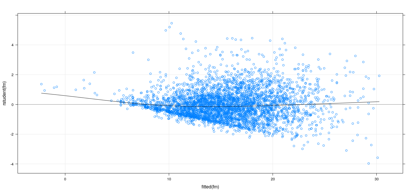
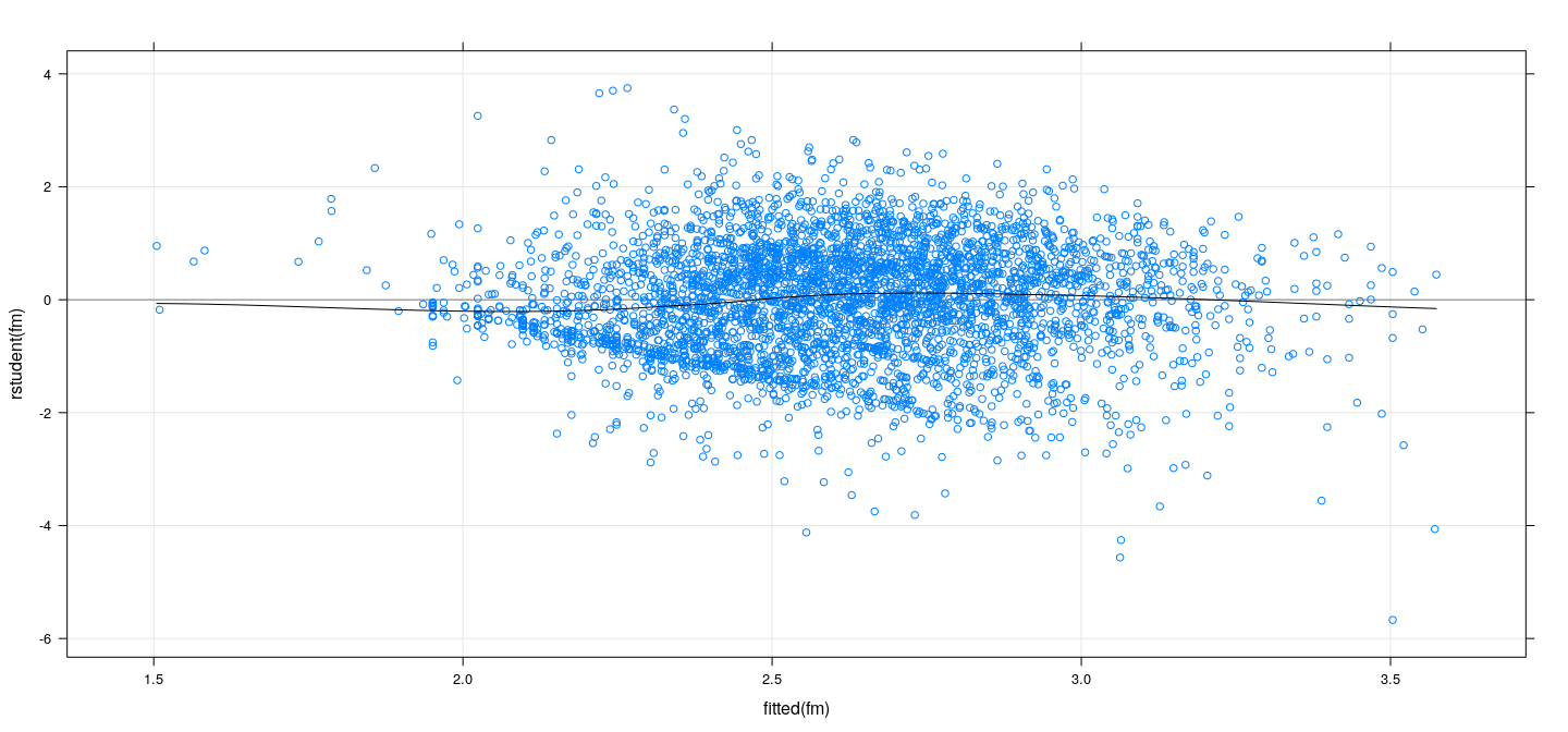
Studentized residuals vs fitted values
![plot of chunk unnamed-chunk-11]()
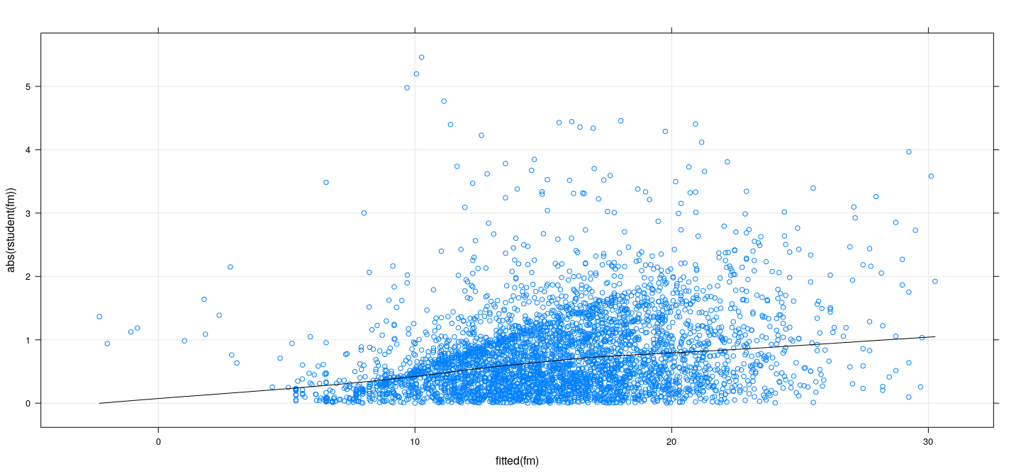
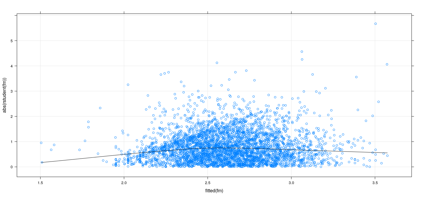
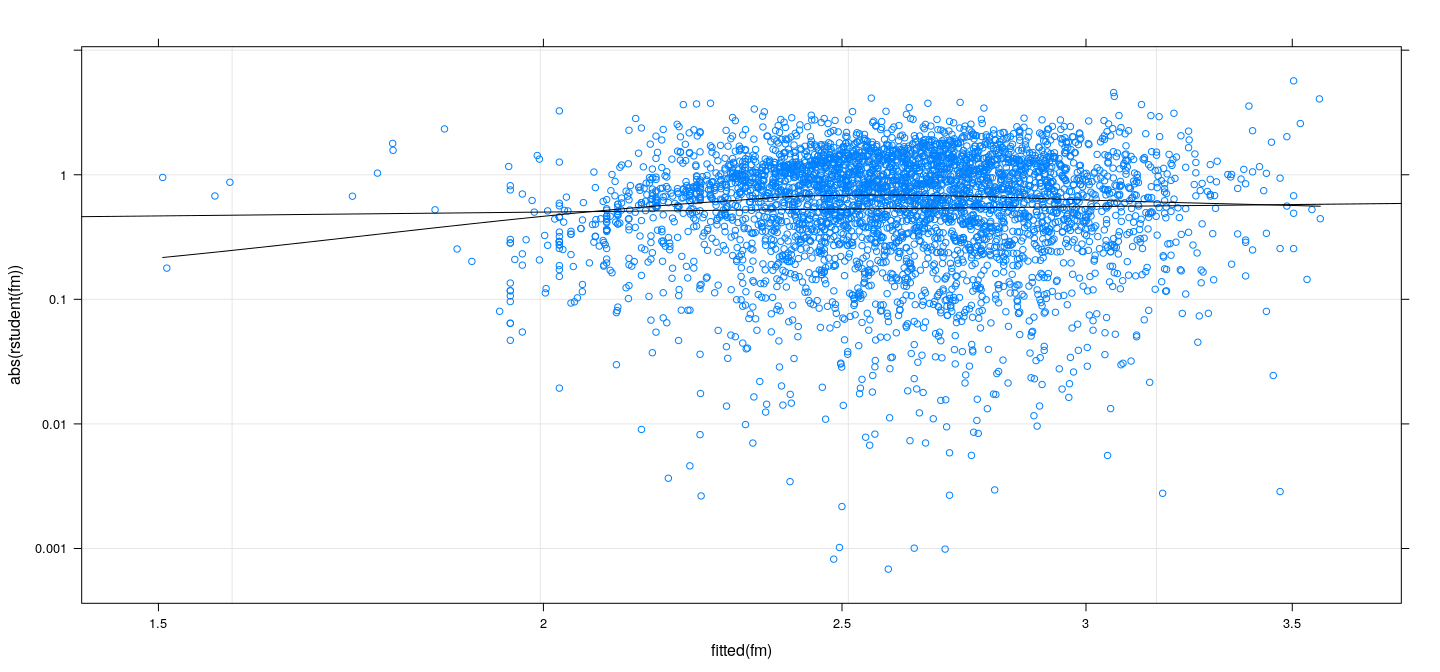
Absolute Studentized residuals vs fitted values
![plot of chunk unnamed-chunk-12]()
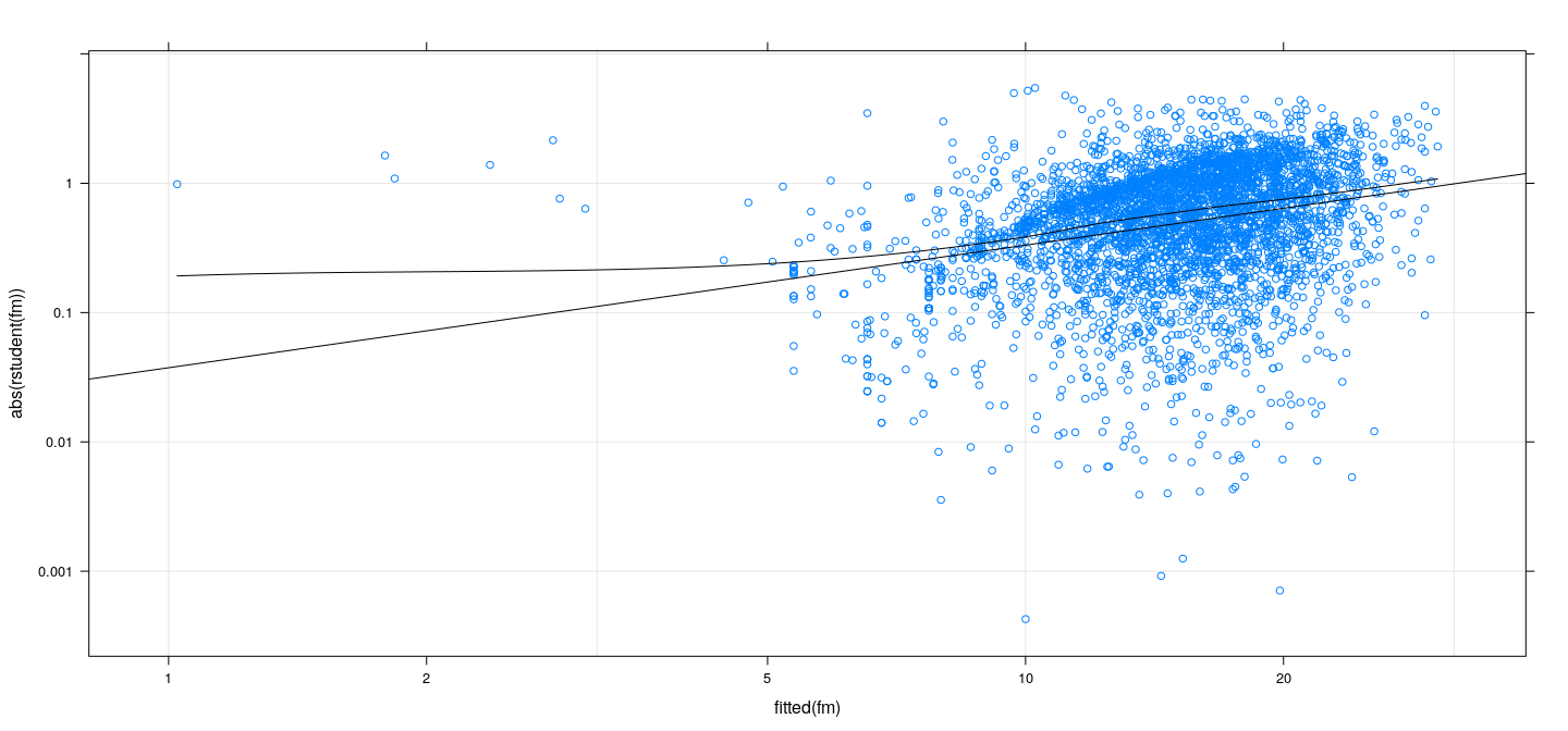
Spread-level plots
Suppose (most) fitted values are positive
We can plot both absolute residuals and fitted values in log scales
A linear relationship in this plot suggests a power transformation
Spread-level plots
![plot of chunk unnamed-chunk-13]()
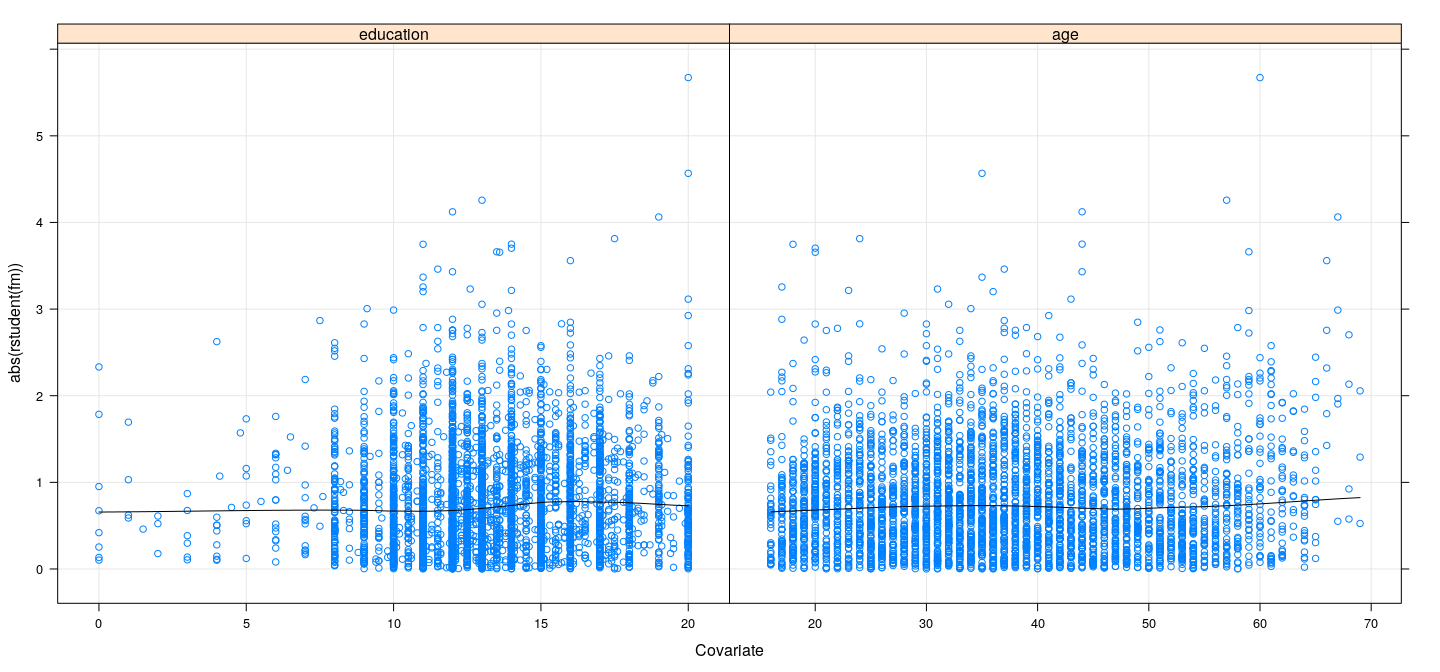
Residuals vs covariates
![plot of chunk unnamed-chunk-18]()
Weighted least-squares estimation
Suppose we can find known weights \(w_i\) such that \(E(y_i | \mathbf{x}_i) = \mathbf{x}_i^T \mathbf{\beta}\) and \(V(y_i | \mathbf{x}_i) = \sigma^2 / w_i^2\)
Let \(\mathbf{W}\) be a diagonal matrix with entries \(w_i^2\) and \(\mathbf{\Sigma} = \sigma^2 \mathbf{W}^{-1}\). Then
\[
\mathbf{y} \sim N( \mathbf{X} \mathbf{\beta}, \mathbf{\Sigma} )
\]
- The likelihood function is given by
\[\begin{align}
L(\mathbf{\beta}, \sigma^2) &=& \frac{1}{(2\pi)^{n/2} \lvert \mathbf{\Sigma} \rvert^{1/2}} \exp \left[ -\frac12 (\mathbf{y} - \mathbf{X} \beta)^T \mathbf{\Sigma}^{-1} (\mathbf{y} - \mathbf{X} \beta) \right] \\
&=& \frac{1}{(2\pi \sigma^2)^{n/2} \lvert \mathbf{W} \rvert^{1/2}} \exp \left[ -\frac1{2\sigma^2} \sum_{i=1}^n w_i^2 (y_i - \mathbf{x}_i^T \beta)^2 \right]
\end{align}\]
Weighted least-squares estimation
- Maximum likelihood estimators are easily seen (exercise) to be given by
\[
\hat{\mathbf{\beta}} = (\mathbf{X}^T \mathbf{W} \mathbf{X})^{-1}
\mathbf{X}^T \mathbf{W} \mathbf{y}\,,\quad
\hat{\sigma}^2 = \frac1{n} \sum w_i^2 (y_i - \mathbf{x}_i^T \hat{\mathbf{\beta}})^2
\]
- In R,
lm() supports weighted least squares through the weights argument
Effect of non-constant variance on OLS estimates
Let \(E(\mathbf{y}) = \mathbf{X} \beta\) and \(V(\mathbf{y}) = \mathbf{\Sigma} = diag\{ \sigma_1^2, \dotsc, \sigma_n^2 \}\)
Suppose we ignore non-constant variance and estimate \(\beta\) using OLS.
\(\hat\beta\) is still unbiased:
\[E(\hat\beta) = (\mathbf{X}^T\mathbf{X})^{-1} \mathbf{X}^T E(\mathbf{y}) = (\mathbf{X}^T\mathbf{X})^{-1} \mathbf{X}^T \mathbf{X} \beta = \beta\]
\[V(\hat\beta) = (\mathbf{X}^T\mathbf{X})^{-1} \mathbf{X}^T \mathbf{\Sigma} \mathbf{X} (\mathbf{X}^T\mathbf{X})^{-1}\]
\[V(\ell^T \hat\beta) = \ell^T (\mathbf{X}^T\mathbf{X})^{-1} \mathbf{X}^T \mathbf{\Sigma} \mathbf{X} (\mathbf{X}^T\mathbf{X})^{-1} \ell\]
- WLS may not be worth the effort if more or less same as OLS standard error
Detecting need for addressing non-constant variance
How can we quickly assess need for WLS?
Suppose we don’t know structural form of \(\mathbf{\Sigma}\) (e.g., which covariates affect variance)
We still know that \(E(\varepsilon_i^2) = \sigma_i^2\)
Natural estimate of \(\sigma_i^2\) after fitting OLS model: \(e_i^2\) or \(e_{i(-i)}^2\), giving \(\hat{\mathbf{\Sigma}}\)
This gives White’s “sandwich estimator”
\[\hat{V}(\hat\beta) = (\mathbf{X}^T\mathbf{X})^{-1} \mathbf{X}^T \hat{\mathbf{\Sigma}} \mathbf{X} (\mathbf{X}^T\mathbf{X})^{-1}\]
How does this help?
We have two alternative estimates of \(V(\hat\beta)\): the OLS and the sandwich estimator
Can obtain corresponding standard errors for \(\ell^T \hat{\beta}\) (in particular for \(t\)-tests for \(\beta_j\)-s)
General strategy:
- If the standard errors using the two methods are substantially similar, OLS is sufficient
- Otherwise, need to address non-constant variance
- This does not suggest any particular remedy: usual approach is to try transformations
How does this help?
Call:
lm(formula = log(wages) ~ education + age + sex, data = SLID)

Residuals:
     Min       1Q   Median       3Q      Max
-2.36252 -0.27716  0.01428  0.28625  1.56588

Coefficients:
             Estimate Std. Error t value Pr(>|t|)
(Intercept) 1.1168632  0.0385480   28.97   <2e-16 ***
education   0.0552139  0.0021891   25.22   <2e-16 ***
age         0.0176334  0.0005476   32.20   <2e-16 ***
sexMale     0.2244032  0.0132238   16.97   <2e-16 ***
---
Signif. codes:  0 '***' 0.001 '**' 0.01 '*' 0.05 '.' 0.1 ' ' 1

Residual standard error: 0.4187 on 4010 degrees of freedom
Multiple R-squared:  0.3094,    Adjusted R-squared:  0.3089
F-statistic: 598.9 on 3 and 4010 DF,  p-value: < 2.2e-16
How does this help?
              (Intercept)     education           age       sexMale
(Intercept)  1.485945e-03 -6.903578e-05 -1.278690e-05 -9.428603e-05
education   -6.903578e-05  4.792018e-06  1.275037e-07  7.454834e-07
age         -1.278690e-05  1.275037e-07  2.999080e-07 -7.403851e-08
sexMale     -9.428603e-05  7.454834e-07 -7.403851e-08  1.748681e-04
 (Intercept)    education          age      sexMale
0.0385479539 0.0021890678 0.0005476385 0.0132237691
How does this help?
              (Intercept)     education           age       sexMale
(Intercept)  1.493908e-03 -7.018477e-05 -1.374008e-05 -7.108659e-05
education   -7.018477e-05  4.946819e-06  1.370821e-07  6.523566e-07
age         -1.374008e-05  1.370821e-07  3.420460e-07 -7.115594e-07
sexMale     -7.108659e-05  6.523566e-07 -7.115594e-07  1.750330e-04
(Intercept)   education         age     sexMale
0.038651104 0.002224144 0.000584847 0.013230005
How does this help?
              (Intercept)     education           age       sexMale
(Intercept)  1.499263e-03 -7.045519e-05 -1.378453e-05 -7.136218e-05
education   -7.045519e-05  4.964996e-06  1.377771e-07  6.614334e-07
age         -1.378453e-05  1.377771e-07  3.430706e-07 -7.121512e-07
sexMale     -7.136218e-05  6.614334e-07 -7.121512e-07  1.753998e-04
 (Intercept)    education          age      sexMale
0.0387203216 0.0022282270 0.0005857223 0.0132438591
Nonlinearity
Non-linearity means the modeled expectation \(E(\mathbf{y}) = \mathbf{X} \beta\) is not adequate
In multiple regression, with many predictors, this may be difficult to detect
Usual strategy: look for indicative patterns in residuals for one predictor at a time
Simplest option is to plot residuals against predictor
But this may not be able to distinguish between monotone and non-monotone relationships
Important to do so because monotone nonlinearity can often be corrected using transformation
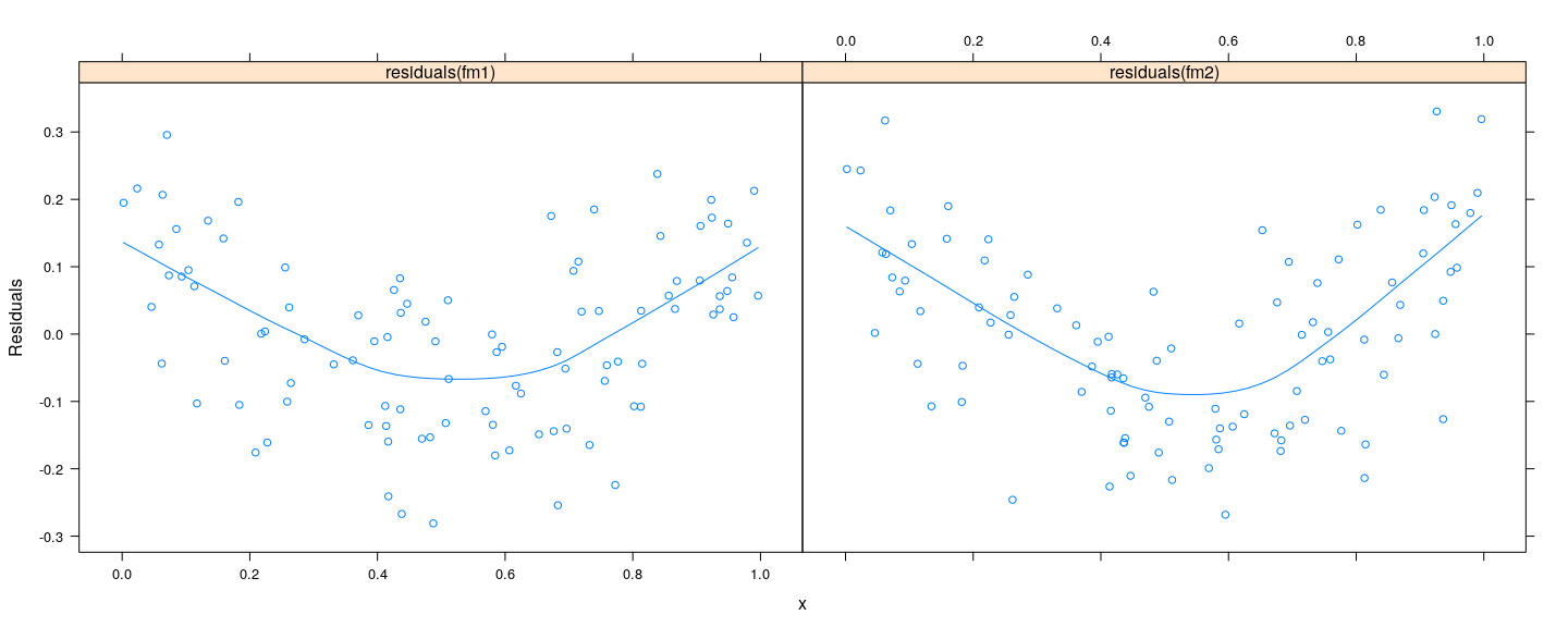
Residual vs covariate: example
![plot of chunk unnamed-chunk-25]()
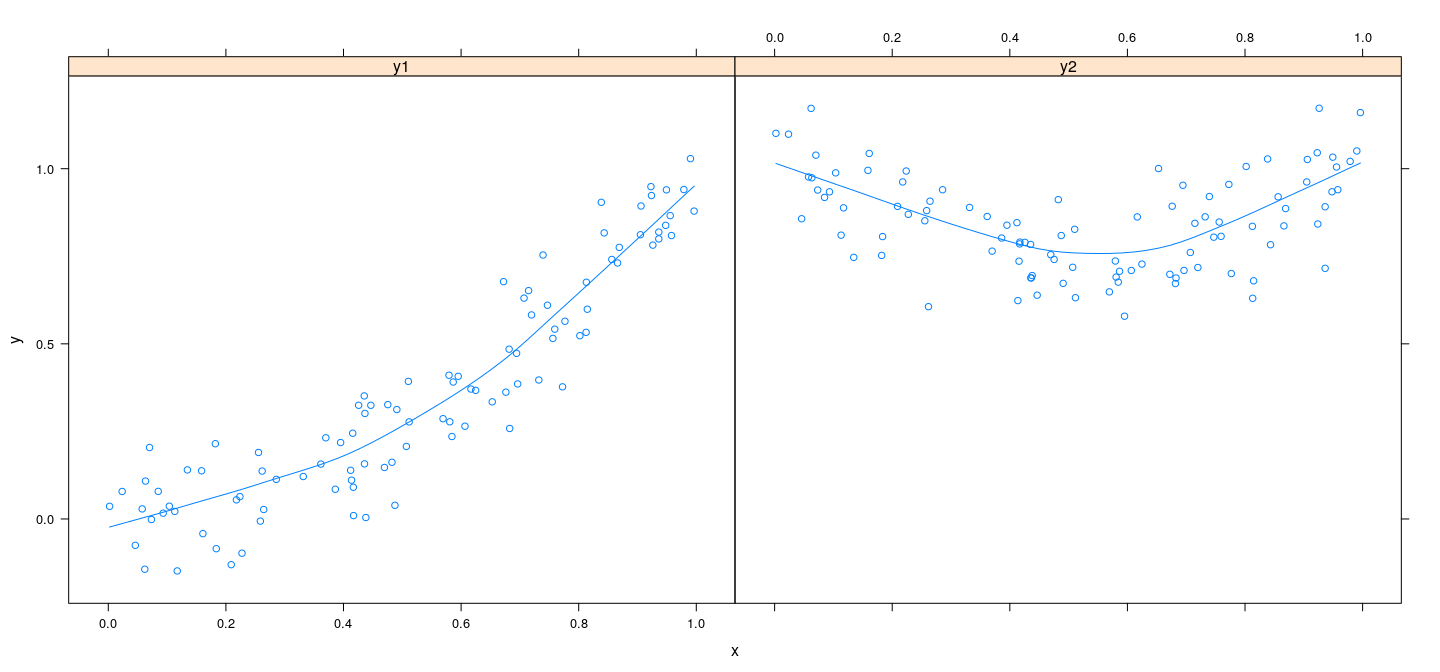
Residual vs covariate: example
- Similar residual plots, but nature of models are different
- First model can be made linear by transformation (true model: \(y = \alpha + \beta x^2 + \varepsilon\))
- Second model is truly quadratic ((true model: \(y = \alpha + \beta x + \gamma x^2 + \varepsilon\))
![plot of chunk unnamed-chunk-26]()
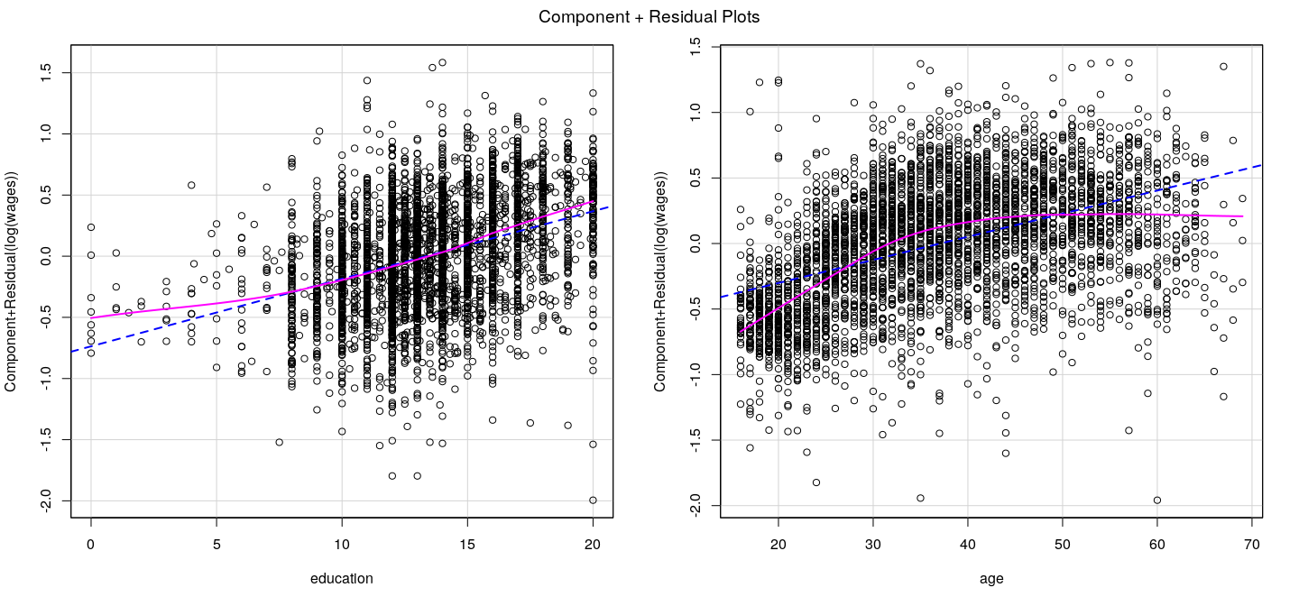
Component plus residual plots
X-axis: \(j\)-th covariate (more accurately, \(j\)-th column of \(\mathbf{X}\))
Y-axis: partial residuals of \(\mathbf{y}\) on \(\mathbf{X}\) excluding \(j\)-th column:
\[e_i^{(-j)} = e_i + \hat{\beta}_j X_{ij}\]
In other words, add back the contribution of the \(j\)-th covariate
Similar to added-variable plots, but covariate is not adjusted
Add non-parametric smoother to detect non-linearity
Component plus residual plots: example
![plot of chunk unnamed-chunk-27]()
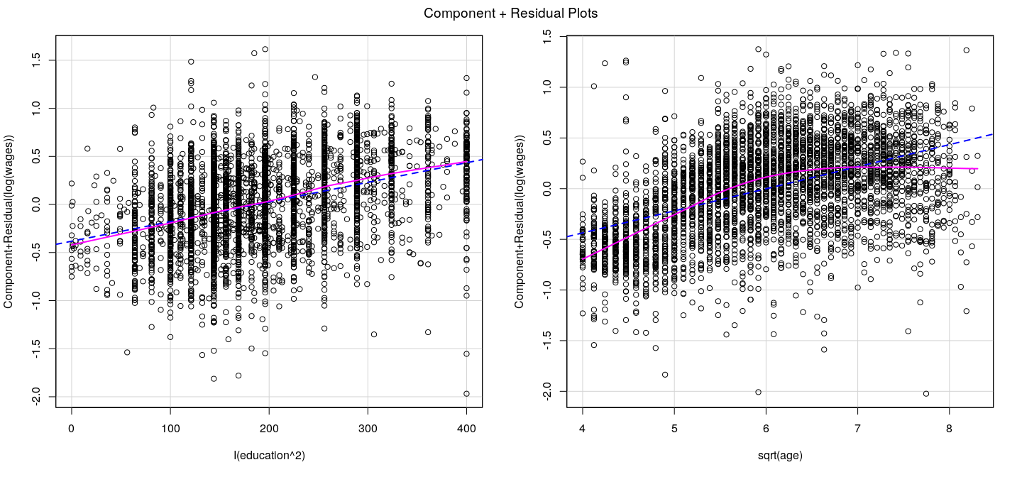
Component plus residual plots: example
![plot of chunk unnamed-chunk-28]()
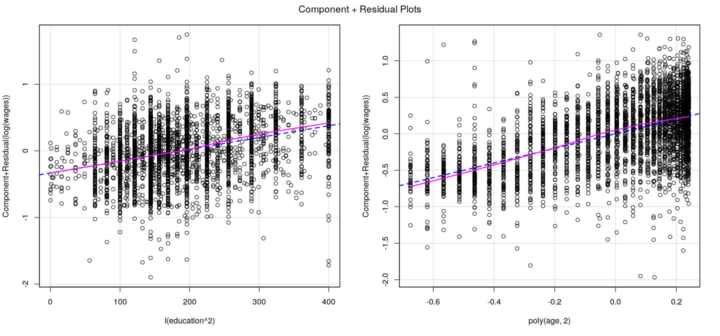
Component plus residual plots: example
![plot of chunk unnamed-chunk-29]()
Component plus residual plots: caveats
Higher dimensional relationships in multiple regression models can be complicated
Component plus residual plots are two dimensional projections
May not always work: in particular, if covariates are non-linearly related
See Mallows (1986) for an approach that accounts for quadratic relationships with other covariates
See Cook (1993) for a more general approach (CERES plots)
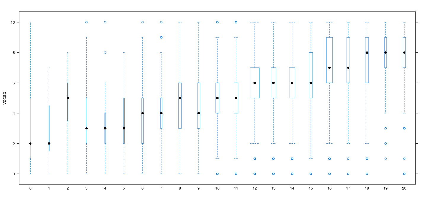
Nonlinearity for discrete predictors
As discussed earlier, discrete covariates (few unique values, many ties) allow us to fit “pure error” models
Pure error models represent a model with no restrictions on the mean function \(f(x) = E(Y | X = x)\)
Can be used to test “lack of fit” for any more specific form of \(f(x)\)
- Example:
GSSvocab (28867 observations)
- Response:
vocab (Number of words out of 10 correct on a vocabulary test)
- Predictors:
age (in years) and educ (years of education)
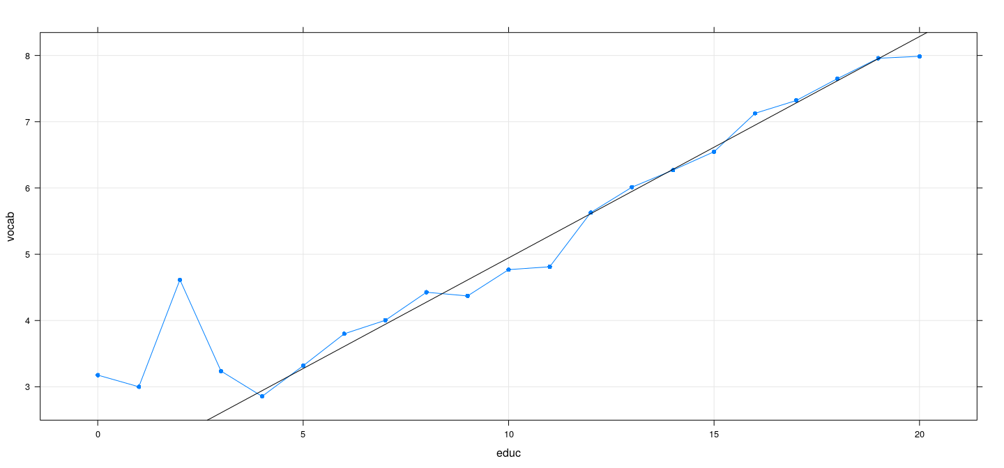
Example: GSSvocab data
![plot of chunk unnamed-chunk-30]()
Example: GSSvocab data
![plot of chunk unnamed-chunk-31]()
Example: GSSvocab data
Analysis of Variance Table

Model 1: vocab ~ educ
Model 2: vocab ~ factor(educ)
  Res.Df   RSS Df Sum of Sq      F    Pr(>F)
1  27471 93895
2  27452 92906 19    989.32 15.386 < 2.2e-16 ***
---
Signif. codes:  0 '***' 0.001 '**' 0.01 '*' 0.05 '.' 0.1 ' ' 1
Example: GSSvocab data
- Even though there is significant lack of fit, the improvement is marginal
[1] 0.2283162
[1] 0.236447
- This is a common theme
- Statistical tests are more sensitive for large \(n\)
- Statistical significance does not necessarily mean the difference (effect) is important in practice
Example: SLID data
- We can do similar tests for multiple regression models
- \(R^2\) does not improve substantially
$fm1
[1] 0.384718

$fm2
[1] 0.4086884

$fm3
[1] 0.3996565

$fm4
[1] 0.423225
Example: SLID data
Analysis of Variance Table

Model 1: log(wages) ~ I(education^2) + poly(age, 2) + sex
Model 2: log(wages) ~ factor(education) + factor(age) + sex
  Res.Df    RSS  Df Sum of Sq      F  Pr(>F)
1   4009 626.42
2   3834 587.21 175    39.204 1.4627 9.9e-05 ***
---
Signif. codes:  0 '***' 0.001 '**' 0.01 '*' 0.05 '.' 0.1 ' ' 1
Example: SLID data
Analysis of Variance Table

Model 1: log(wages) ~ factor(education) + poly(age, 2) + sex
Model 2: log(wages) ~ factor(education) + factor(age) + sex
  Res.Df    RSS Df Sum of Sq      F    Pr(>F)
1   3885 602.01
2   3834 587.21 51      14.8 1.8947 0.0001394 ***
---
Signif. codes:  0 '***' 0.001 '**' 0.01 '*' 0.05 '.' 0.1 ' ' 1
Analysis of Variance Table

Model 1: log(wages) ~ I(education^2) + factor(age) + sex
Model 2: log(wages) ~ factor(education) + factor(age) + sex
  Res.Df    RSS  Df Sum of Sq      F  Pr(>F)
1   3958 611.21
2   3834 587.21 124    23.995 1.2634 0.02743 *
---
Signif. codes:  0 '***' 0.001 '**' 0.01 '*' 0.05 '.' 0.1 ' ' 1
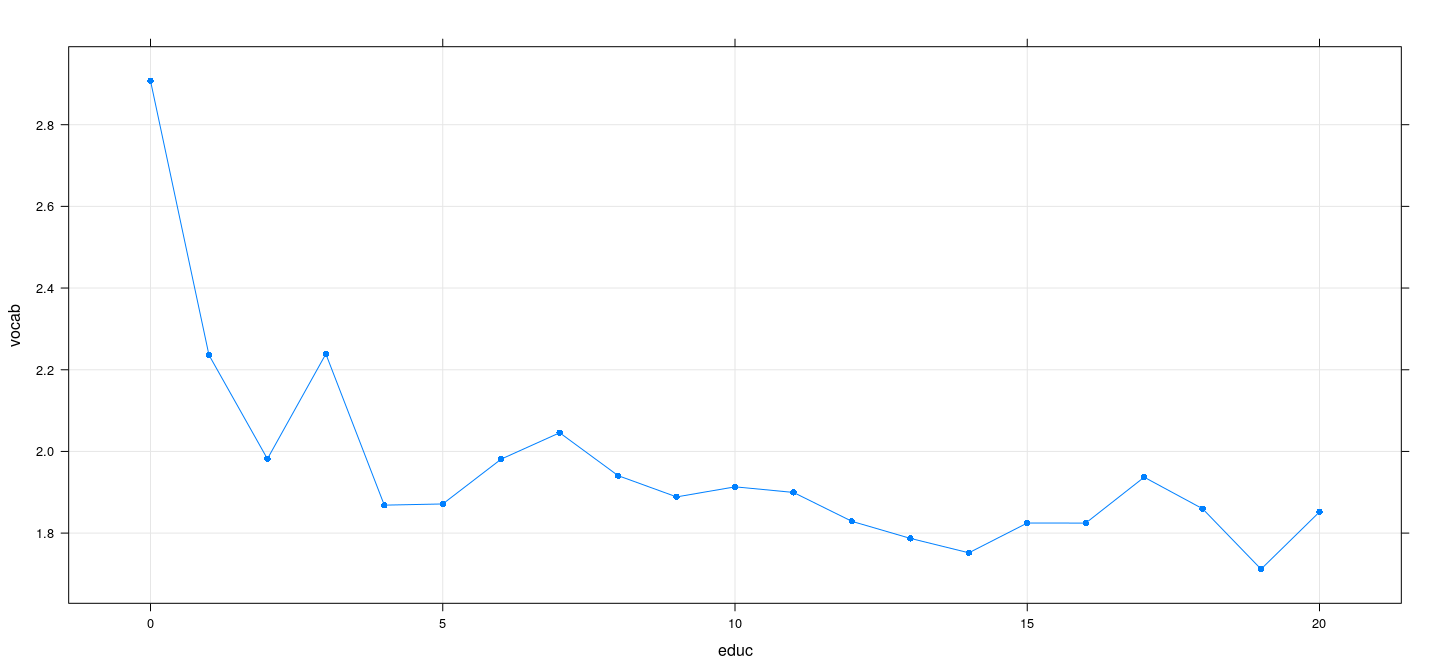
Using pure error models to test for non-constant variance
- With discrete predictors, constant variance means within-group sample variances should be similar
\[
S_j^2 = \frac{1}{n_j-1} \sum_{i=1}^{n_j} (y_{ij} - \bar{y}_j)^2, j = 1, \dotsc, k
\]
- Define the pooled variance
\[
S_p^2 = \frac{1}{n-k} \sum_{j=1}^k (n_j - 1) S_j^2, \text{ where } n = \sum_{j=1}^k n_j
\]
- Then Bartlett’s test statistic is (an adjustment of the likelihood ratio test statistic)
\[
T = \frac{(n-k) \log S_p^2 - \sum_{j=1}^k (n_j-1) \log S_j^2 }{1 + \frac{1}{3(k-1)} (\sum_{j=1}^k \frac{1}{n_j - 1} - \frac{1}{n-k})}
\]
- Under the null distribution of constant variance, \(T\) follows a \(\chi^2\) distribution with \((k-1)\) d.f.
Using pure error models to test for non-constant variance
![plot of chunk unnamed-chunk-39]()
Using pure error models to test for non-constant variance
    Bartlett test of homogeneity of variances

data:  vocab by factor(educ)
Bartlett's K-squared = 78.606, df = 20, p-value = 6.761e-09
Levene's Test for Homogeneity of Variance (center = median)
         Df F value   Pr(>F)
group    20  5.3673 6.42e-14 ***
      27452
---
Signif. codes:  0 '***' 0.001 '**' 0.01 '*' 0.05 '.' 0.1 ' ' 1
The Box-Tidwell procedure: example
                    MLE of lambda Score Statistic (z)  Pr(>|z|)
I(0.01 + education)        1.8696               4.396 1.103e-05 ***
age                       -1.6301             -21.772 < 2.2e-16 ***
---
Signif. codes:  0 '***' 0.001 '**' 0.01 '*' 0.05 '.' 0.1 ' ' 1

iterations =  9