An overview of the R programming environment
Deepayan Sarkar
Software for Statistics
Computing software is essential for modern statistics
Large datasets
Visualization
Simulation
Iterative methods
Many softwares are available
We will learn about R
Available as Free / Open Source Software
Very popular (both academia and industry)
Easy to try out on your own
Outline
Installing R
Some examples
A little bit of history
Some thoughts on why R has been successful
Installing R
R is most commonly used as a REPL (Read-Eval-Print-Loop)
This is essentially the model used by a calculator:
Waits for user input
Evaluates and prints result
Waits for more input
There are several different interfaces to do this
R itself works on many platforms (Windows, Mac, UNIX, Linux)
Some interfaces are platform-specific, some work on most
- R and the interface may need to be installed separately
Installing R
Go to https://cran.r-project.org/ (or choose a mirror first)
Follow instructions depending on your platform (probably Windows)
- This will install R, as well as a default graphical interface on Windows and Mac
I will recommend a different interface called R Studio that needs to be installed separately
I personally use yet another interface called ESS which works with a general purpose editor called Emacs (download link for Windows)
Running R
- Once installed, you can start the appropriate interface (or R directly) to get something like this:
R Under development (unstable) (2018-05-05 r74699) -- "Unsuffered Consequences"
Copyright (C) 2018 The R Foundation for Statistical Computing
Platform: x86_64-pc-linux-gnu (64-bit)

R is free software and comes with ABSOLUTELY NO WARRANTY.
You are welcome to redistribute it under certain conditions.
Type 'license()' or 'licence()' for distribution details.

  Natural language support but running in an English locale

R is a collaborative project with many contributors.
Type 'contributors()' for more information and
'citation()' on how to cite R or R packages in publications.

Type 'demo()' for some demos, 'help()' for on-line help, or
'help.start()' for an HTML browser interface to help.
Type 'q()' to quit R.

Loading required package: utils
>
The
>represents a prompt indicating that R is waiting for input.The difficult part is to learn what to do next
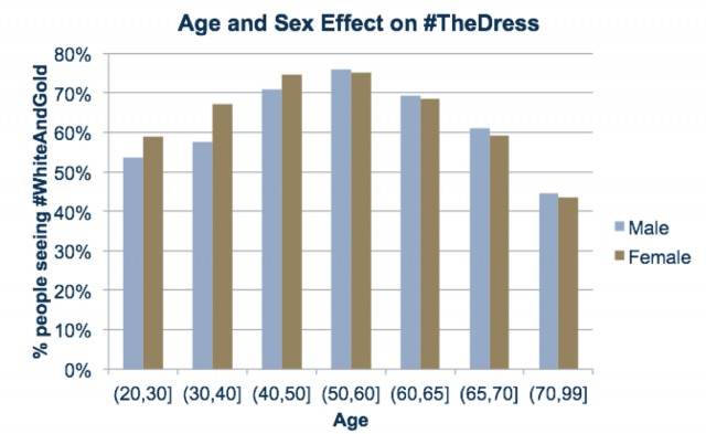
Before we start, an experiment!

Color combination: Is it white & gold or blue & black ? Let’s count!
Question: What proportion of population sees white & gold?
Statistics uses data to make inferences
Model:
Let \(p\) be the probability of seeing white & gold
Assume that individuals are independent
Data:
Suppose \(X\) out of \(N\) sampled individuals see white & gold; e.g., \(N = 44\), \(X = 26\).
According to model, \(X \sim Bin(N, p)\)
“Obvious” estimate of \(p = X / N = 26 / 44 = 0.5909\)
But how is this estimate derived?
Generally useful method: maximum likelihood
- Likelihood function: probability of observed data as function of \(p\)
\[ L(p) = P(X = 26) = {44 \choose 26} p^{26} (1-p)^{(44-26)}, p \in (0, 1) \]
Intuition: \(p\) that gives higher \(L(p)\) is more “likely” to be correct
Maximum likelihood estimate \(\hat{p} = \arg \max L(p)\)
- By differentiating \[ \log L(p) = c + 26 \log p + 18 \log (1-p) \] we get \[ \frac{d}{dp} \log L(p) = \frac{26}{p} - \frac{18}{1-p} = 0 \implies 26 (1-p) - 18 p = 0 \implies p = \frac{26}{44} \]
How could we do this numerically?
Pretend for the moment that we did not know how to do this.
How could we arrive at the same solution numerically?
Basic idea: Compute \(L(p)\) for various values of \(p\) and find minimum.
To do this in R, the most important thing to understand is that R works like a calculator:
The user types in an expression, R calculates the answer
The expression can involve numbers, variables, and functions
“Vectorized” computations
- One distinguishing feature of R is that it operates on “vectors”
  [1] 0.00 0.01 0.02 0.03 0.04 0.05 0.06 0.07 0.08 0.09 0.10 0.11 0.12 0.13 0.14 0.15 0.16 0.17 0.18 0.19 0.20 0.21 0.22
 [24] 0.23 0.24 0.25 0.26 0.27 0.28 0.29 0.30 0.31 0.32 0.33 0.34 0.35 0.36 0.37 0.38 0.39 0.40 0.41 0.42 0.43 0.44 0.45
 [47] 0.46 0.47 0.48 0.49 0.50 0.51 0.52 0.53 0.54 0.55 0.56 0.57 0.58 0.59 0.60 0.61 0.62 0.63 0.64 0.65 0.66 0.67 0.68
 [70] 0.69 0.70 0.71 0.72 0.73 0.74 0.75 0.76 0.77 0.78 0.79 0.80 0.81 0.82 0.83 0.84 0.85 0.86 0.87 0.88 0.89 0.90 0.91
[93] 0.92 0.93 0.94 0.95 0.96 0.97 0.98 0.99 1.00 [1] 0.000000e+00 8.591575e-41 4.802734e-33 1.512457e-28 2.223726e-25 6.093745e-23 5.765981e-21 2.617468e-19
[9] 6.936811e-18 1.218119e-16 1.545270e-15 1.506153e-14 1.180429e-13 7.700395e-13 4.294774e-12 2.091957e-11
[17] 9.052864e-11 3.529530e-10 1.254220e-09 4.101694e-09 1.244626e-08 3.528813e-08 9.404416e-08 2.368078e-07
[25] 5.659476e-07 1.288790e-06 2.806191e-06 5.860149e-06 1.176882e-05 2.278440e-05 4.261443e-05 7.714841e-05
[33] 1.354251e-04 2.308597e-04 3.827207e-04 6.178014e-04 9.721737e-04 1.492843e-03 2.239047e-03 3.282888e-03
[41] 4.708923e-03 6.612349e-03 9.095461e-03 1.226215e-02 1.621039e-02 2.102292e-02 2.675658e-02 3.343099e-02
[49] 4.101773e-02 4.943113e-02 5.852204e-02 6.807589e-02 7.781593e-02 8.741246e-02 9.649794e-02 1.046874e-01
[57] 1.116031e-01 1.169009e-01 1.202969e-01 1.215909e-01 1.206845e-01 1.175920e-01 1.124418e-01 1.054689e-01
[65] 9.699819e-02 8.742011e-02 7.716176e-02 6.665536e-02 5.630807e-02 4.647572e-02 3.744302e-02 2.941171e-02
[73] 2.249722e-02 1.673329e-02 1.208326e-02 8.455753e-03 5.722622e-03 3.736794e-03 2.348049e-03 1.415438e-03
[81] 8.156783e-04 4.475222e-04 2.326508e-04 1.139594e-04 5.224689e-05 2.224201e-05 8.707704e-06 3.098277e-06
[89] 9.873047e-07 2.765972e-07 6.651882e-08 1.330702e-08 2.121986e-09 2.540743e-10 2.092599e-11 1.034935e-12
[97] 2.447773e-14 1.806704e-16 1.596089e-19 7.927831e-25 0.000000e+00Plotting is very easy

Functions
Functions can be used to encapsulate repetitive computations
Like mathematical functions, R function also take arguments as input and “returns” an output
[1] 0.05852204[1] 0.1216Functions can be plotted directly

…and they can be numerically “optimized”
$maximum
[1] 0.5909084

$objective
[1] 0.1216
- Compare with
[1] 0.5909091A more complicated example
Suppose \(X_1, X_2, ..., X_n \sim Bin(N, p)\), and are independent
Instead of observing each \(X_i\), we only get to know \(M = \max(X_1, X_2, ..., X_n)\)
What is the maximum likelihood estimate of \(p\)? (\(N\) and \(n\) are known, \(M = m\) is observed)
A more complicated example
To compute likelihood, we need p.m.f. of \(M\) : \[ P(M \leq m) = P(X_1 \leq m, ..., X_n \leq m) = \left[ \sum_{x=0}^m {N \choose x} p^{x} (1-p)^{(N-x)} \right]^n \] and \[ P(M = m) = P(M \leq m) - P(M \leq m-1) \]
Maximum Likelihood estimate

$maximum
[1] 0.4996703

$objective
[1] 0.1981222
“The Dress” revisited
- What factors determine perceived color? (From 23andme.com)
Simulation: birthday problem
R can be used to simulate random events
Example: how likely is a common birthday in a group of 20 people?
[1] 112 320 19 42 66 41 73 182 314 266 154 313 351 276 218 359 257 246 195 42[1] 19Law of Large Numbers
- With enough replications, sample proportion should converge to probability
[1] FALSE[1] FALSE[1] TRUE[1] TRUELaw of Large Numbers
With enough replications, sample proportion should converge to probability
Do this sytematically:
  [1] FALSE FALSE FALSE  TRUE FALSE FALSE  TRUE  TRUE  TRUE FALSE  TRUE FALSE FALSE FALSE  TRUE  TRUE FALSE  TRUE  TRUE
 [20]  TRUE FALSE  TRUE  TRUE  TRUE FALSE FALSE  TRUE FALSE FALSE FALSE  TRUE FALSE  TRUE FALSE  TRUE  TRUE FALSE FALSE
 [39]  TRUE FALSE FALSE  TRUE  TRUE FALSE  TRUE FALSE FALSE  TRUE  TRUE FALSE  TRUE  TRUE FALSE  TRUE FALSE FALSE FALSE
 [58]  TRUE FALSE  TRUE FALSE FALSE FALSE FALSE  TRUE FALSE  TRUE FALSE FALSE  TRUE FALSE FALSE FALSE  TRUE FALSE FALSE
 [77] FALSE  TRUE  TRUE FALSE FALSE FALSE  TRUE FALSE  TRUE FALSE FALSE FALSE FALSE  TRUE FALSE FALSE  TRUE FALSE FALSE
 [96] FALSE  TRUE FALSE FALSE FALSE
Law of Large Numbers
- With enough replications, sample proportion should converge to probability
plot(cumsum(replicate(1000, haveCommon())) / 1:1000, type = "l")
lines(cumsum(replicate(1000, haveCommon())) / 1:1000, col = "red")
lines(cumsum(replicate(1000, haveCommon())) / 1:1000, col = "blue")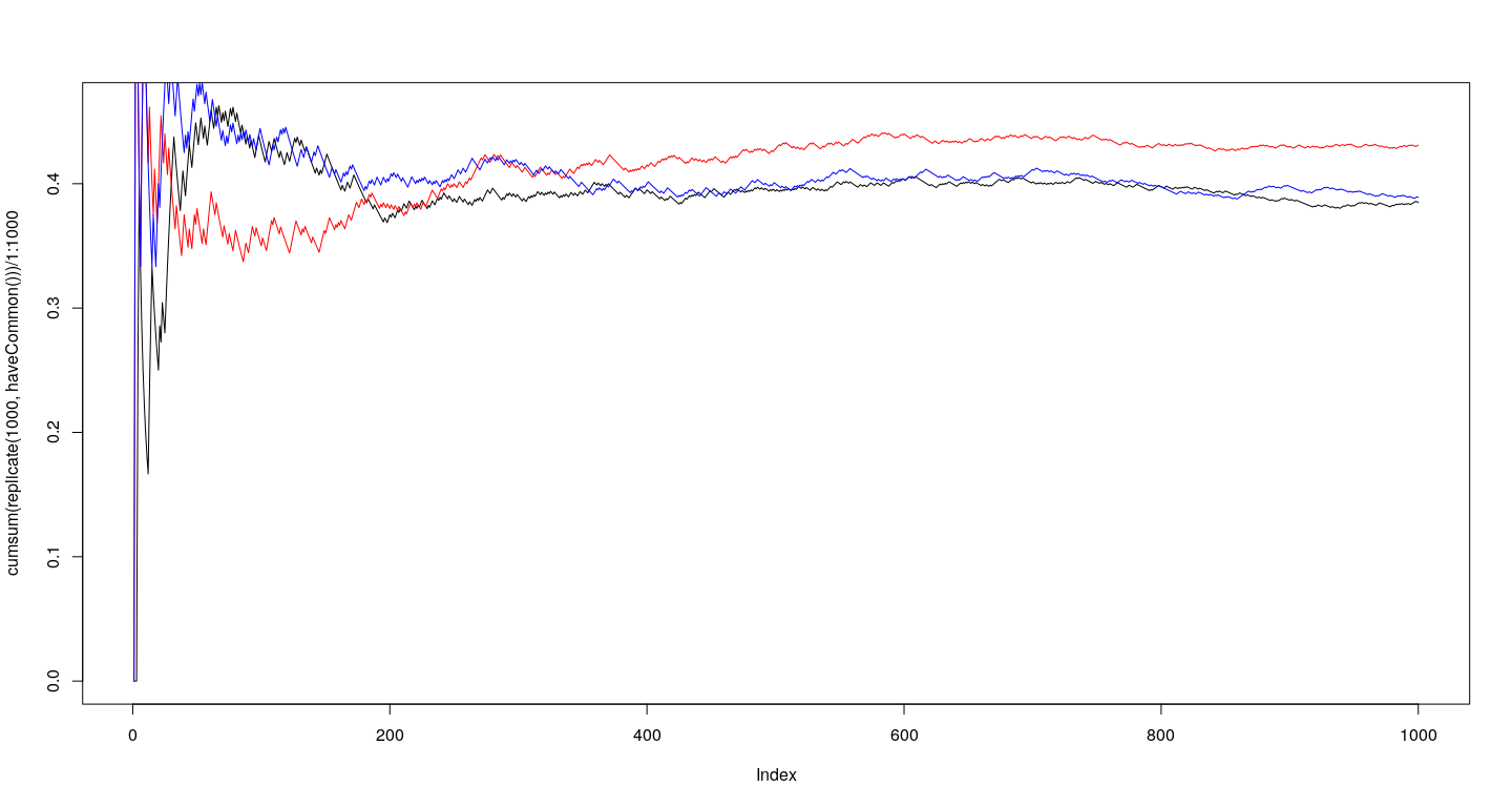
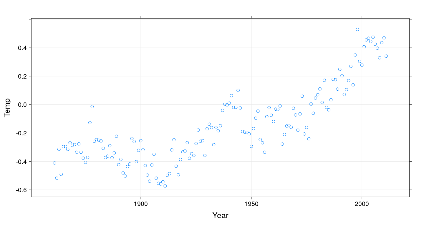
A more serious example: climate change
| Year | Temp | CO2 | CH4 | NO2 |
|---|---|---|---|---|
| 1861 | -0.411 | 286.5 | 838.2 | 288.9 |
| 1862 | -0.518 | 286.6 | 839.6 | 288.9 |
| 1863 | -0.315 | 286.8 | 840.9 | 289.0 |
| 1864 | -0.491 | 287.0 | 842.3 | 289.1 |
| 1865 | -0.296 | 287.2 | 843.8 | 289.1 |
| 1866 | -0.295 | 287.4 | 845.5 | 289.2 |
| 1867 | -0.315 | 287.6 | 847.1 | 289.3 |
| 1868 | -0.268 | 287.8 | 848.6 | 289.3 |
| 1869 | -0.287 | 288.0 | 850.2 | 289.4 |
| 1870 | -0.282 | 288.2 | 851.8 | 289.5 |
| 1871 | -0.335 | 288.4 | 853.4 | 289.5 |
| 1872 | -0.277 | 288.7 | 855.1 | 289.6 |
| 1873 | -0.335 | 288.9 | 856.9 | 289.7 |
| 1874 | -0.377 | 289.1 | 858.8 | 289.7 |
| 1875 | -0.406 | 289.4 | 860.5 | 289.8 |
| 1876 | -0.372 | 289.7 | 862.3 | 289.9 |
| 1877 | -0.127 | 289.9 | 864.0 | 290.0 |
| 1878 | -0.014 | 290.2 | 865.8 | 290.0 |
| 1879 | -0.258 | 290.5 | 867.6 | 290.1 |
| 1880 | -0.247 | 290.8 | 869.4 | 290.2 |
| 1881 | -0.251 | 291.1 | 871.2 | 290.3 |
| 1882 | -0.256 | 291.4 | 872.9 | 290.3 |
| 1883 | -0.308 | 291.7 | 874.7 | 290.4 |
| 1884 | -0.373 | 292.0 | 876.5 | 290.5 |
| 1885 | -0.363 | 292.3 | 878.3 | 290.6 |
| 1886 | -0.289 | 292.6 | 880.0 | 290.7 |
| 1887 | -0.374 | 292.9 | 881.8 | 290.8 |
| 1888 | -0.340 | 293.1 | 883.6 | 290.8 |
| 1889 | -0.223 | 293.4 | 885.4 | 290.9 |
| 1890 | -0.423 | 293.7 | 887.2 | 291.0 |
| 1891 | -0.386 | 294.0 | 888.9 | 291.1 |
| 1892 | -0.481 | 294.3 | 890.6 | 291.2 |
| 1893 | -0.503 | 294.6 | 892.2 | 291.3 |
| 1894 | -0.436 | 294.9 | 893.9 | 291.4 |
| 1895 | -0.418 | 295.2 | 895.6 | 291.4 |
| 1896 | -0.239 | 295.5 | 897.2 | 291.5 |
| 1897 | -0.260 | 295.8 | 898.9 | 291.6 |
| 1898 | -0.402 | 296.1 | 900.5 | 291.7 |
| 1899 | -0.322 | 296.4 | 902.2 | 291.8 |
| 1900 | -0.254 | 296.7 | 903.8 | 291.9 |
| 1901 | -0.317 | 297.0 | 905.5 | 292.0 |
| 1902 | -0.429 | 297.3 | 907.2 | 292.1 |
| 1903 | -0.496 | 297.6 | 908.8 | 292.2 |
| 1904 | -0.539 | 297.9 | 910.5 | 292.3 |
| 1905 | -0.425 | 298.2 | 912.1 | 292.4 |
| 1906 | -0.350 | 298.5 | 913.8 | 292.5 |
| 1907 | -0.518 | 298.9 | 915.4 | 292.6 |
| 1908 | -0.554 | 299.2 | 917.1 | 292.7 |
| 1909 | -0.559 | 299.6 | 918.8 | 292.8 |
| 1910 | -0.544 | 299.9 | 920.4 | 292.9 |
| 1911 | -0.573 | 300.2 | 922.1 | 293.0 |
| 1912 | -0.497 | 300.5 | 924.9 | 293.1 |
| 1913 | -0.486 | 300.9 | 927.8 | 293.2 |
| 1914 | -0.319 | 301.2 | 930.6 | 293.3 |
| 1915 | -0.247 | 301.5 | 933.5 | 293.5 |
| 1916 | -0.434 | 301.8 | 936.4 | 293.6 |
| 1917 | -0.494 | 302.2 | 939.2 | 293.7 |
| 1918 | -0.387 | 302.5 | 942.8 | 293.8 |
| 1919 | -0.332 | 302.9 | 946.3 | 293.9 |
| 1920 | -0.327 | 303.2 | 949.9 | 294.0 |
| 1921 | -0.268 | 303.5 | 953.5 | 294.1 |
| 1922 | -0.378 | 303.9 | 957.1 | 294.2 |
| 1923 | -0.346 | 304.2 | 960.7 | 294.4 |
| 1924 | -0.358 | 304.6 | 964.2 | 294.5 |
| 1925 | -0.274 | 304.9 | 967.8 | 294.6 |
| 1926 | -0.179 | 305.2 | 971.3 | 294.7 |
| 1927 | -0.258 | 305.6 | 974.9 | 294.8 |
| 1928 | -0.254 | 305.9 | 978.5 | 295.0 |
| 1929 | -0.358 | 306.2 | 982.1 | 295.1 |
| 1930 | -0.170 | 306.5 | 985.7 | 295.2 |
| 1931 | -0.138 | 306.8 | 989.2 | 295.3 |
| 1932 | -0.162 | 307.1 | 993.5 | 295.5 |
| 1933 | -0.282 | 307.4 | 997.7 | 295.6 |
| 1934 | -0.161 | 307.7 | 1002.0 | 295.7 |
| 1935 | -0.184 | 308.0 | 1006.2 | 295.9 |
| 1936 | -0.149 | 308.3 | 1010.4 | 296.0 |
| 1937 | -0.041 | 308.5 | 1014.7 | 296.1 |
| 1938 | 0.002 | 308.8 | 1018.9 | 296.3 |
| 1939 | -0.002 | 309.1 | 1023.2 | 296.4 |
| 1940 | 0.010 | 309.3 | 1027.4 | 296.5 |
| 1941 | 0.063 | 309.5 | 1032.2 | 296.7 |
| 1942 | -0.020 | 309.8 | 1037.9 | 296.8 |
| 1943 | -0.019 | 310.0 | 1044.4 | 297.0 |
| 1944 | 0.100 | 310.2 | 1051.7 | 297.1 |
| 1945 | -0.024 | 310.5 | 1059.7 | 297.2 |
| 1946 | -0.189 | 310.8 | 1068.4 | 297.4 |
| 1947 | -0.194 | 311.0 | 1077.8 | 297.5 |
| 1948 | -0.196 | 311.3 | 1087.9 | 297.7 |
| 1949 | -0.206 | 311.7 | 1098.6 | 297.8 |
| 1950 | -0.294 | 312.0 | 1109.9 | 298.0 |
| 1951 | -0.169 | 312.4 | 1121.8 | 298.1 |
| 1952 | -0.096 | 312.8 | 1134.2 | 298.3 |
| 1953 | -0.046 | 313.2 | 1147.1 | 298.4 |
| 1954 | -0.246 | 313.6 | 1160.4 | 298.6 |
| 1955 | -0.269 | 314.1 | 1174.3 | 298.7 |
| 1956 | -0.335 | 314.6 | 1188.5 | 298.9 |
| 1957 | -0.085 | 315.1 | 1203.2 | 299.0 |
| 1958 | -0.021 | 315.2 | 1218.2 | 299.2 |
| 1959 | -0.075 | 316.0 | 1233.5 | 299.4 |
| 1960 | -0.119 | 316.9 | 1249.1 | 299.5 |
| 1961 | -0.032 | 317.6 | 1265.0 | 299.7 |
| 1962 | -0.034 | 318.5 | 1281.1 | 299.8 |
| 1963 | -0.010 | 319.0 | 1297.5 | 300.0 |
| 1964 | -0.278 | 319.6 | 1314.0 | 300.2 |
| 1965 | -0.211 | 320.0 | 1330.7 | 300.3 |
| 1966 | -0.151 | 321.4 | 1347.4 | 300.5 |
| 1967 | -0.147 | 322.2 | 1364.3 | 300.7 |
| 1968 | -0.160 | 323.0 | 1381.2 | 300.8 |
| 1969 | -0.026 | 324.6 | 1398.2 | 301.0 |
| 1970 | -0.073 | 325.7 | 1415.1 | 301.2 |
| 1971 | -0.180 | 326.3 | 1432.1 | 301.4 |
| 1972 | -0.066 | 327.5 | 1448.9 | 301.5 |
| 1973 | 0.059 | 329.7 | 1465.7 | 301.7 |
| 1974 | -0.207 | 330.2 | 1482.4 | 301.9 |
| 1975 | -0.161 | 331.1 | 1498.9 | 302.1 |
| 1976 | -0.241 | 332.1 | 1515.2 | 302.3 |
| 1977 | 0.004 | 333.8 | 1531.3 | 302.4 |
| 1978 | -0.061 | 335.4 | 1547.1 | 302.6 |
| 1979 | 0.046 | 336.8 | 1562.7 | 302.8 |
| 1980 | 0.069 | 338.7 | 1578.0 | 300.7 |
| 1981 | 0.110 | 340.1 | 1593.0 | 301.3 |
| 1982 | 0.015 | 341.4 | 1607.6 | 302.7 |
| 1983 | 0.171 | 343.0 | 1621.8 | 303.1 |
| 1984 | -0.019 | 344.6 | 1653.2 | 303.5 |
| 1985 | -0.037 | 346.0 | 1665.7 | 304.0 |
| 1986 | 0.034 | 347.4 | 1678.3 | 305.0 |
| 1987 | 0.178 | 349.2 | 1690.6 | 305.7 |
| 1988 | 0.175 | 351.6 | 1701.8 | 306.6 |
| 1989 | 0.109 | 353.1 | 1712.6 | 307.6 |
| 1990 | 0.248 | 354.3 | 1722.3 | 307.6 |
| 1991 | 0.203 | 355.6 | 1733.4 | 308.7 |
| 1992 | 0.071 | 356.4 | 1742.2 | 309.4 |
| 1993 | 0.105 | 357.1 | 1744.9 | 310.0 |
| 1994 | 0.169 | 358.8 | 1750.2 | 310.9 |
| 1995 | 0.269 | 360.8 | 1757.2 | 311.4 |
| 1996 | 0.139 | 362.6 | 1760.3 | 312.2 |
| 1997 | 0.349 | 363.7 | 1763.6 | 313.1 |
| 1998 | 0.529 | 366.7 | 1772.9 | 313.9 |
| 1999 | 0.304 | 368.3 | 1781.0 | 314.7 |
| 2000 | 0.278 | 369.5 | 1781.9 | 315.7 |
| 2001 | 0.407 | 371.1 | 1781.0 | 316.4 |
| 2002 | 0.455 | 373.2 | 1782.3 | 317.1 |
| 2003 | 0.467 | 375.8 | 1786.2 | 317.7 |
| 2004 | 0.444 | 377.5 | 1785.5 | 318.4 |
| 2005 | 0.474 | 379.8 | 1784.6 | 319.1 |
| 2006 | 0.425 | 381.9 | 1784.5 | 320.0 |
| 2007 | 0.397 | 383.8 | 1790.4 | 320.8 |
| 2008 | 0.329 | 385.6 | 1797.8 | 321.7 |
| 2009 | 0.436 | 387.4 | 1802.7 | 322.4 |
| 2010 | 0.470 | 389.8 | 1807.7 | 323.2 |
| 2011 | 0.341 | 391.6 | 1813.1 | 324.2 |
Change in temperature (global average deviation) since 1851
Change in atmospheric carbon dioxide
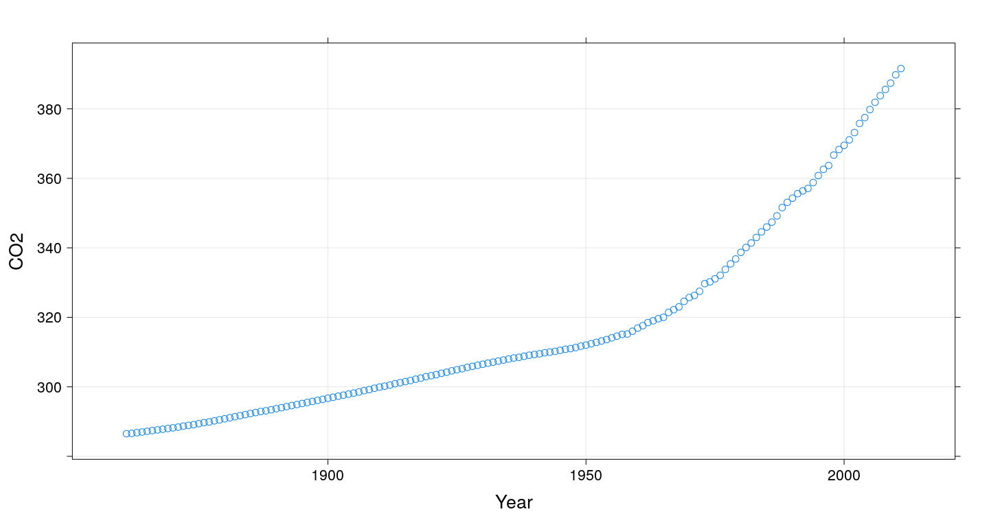
Does change in \(CO_2\) explain temperature rise?
xyplot(Temp ~ CO2, data = globalTemp, grid = TRUE, type = c("p", "r")) # include OLS regression line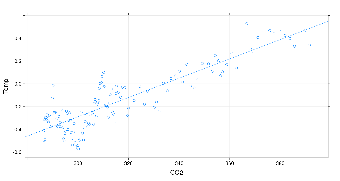
Fitting the regression model
 (Intercept)          CO2
-2.836082117  0.008486628
We can confirm using a general optimizer:
SSE = function(beta)
{
    with(globalTemp,
         sum((Temp - beta[1] - beta[2] * CO2)^2))
}
optim(c(0, 0), fn = SSE)
$par
[1] -2.836176636 0.008486886
$value
[1] 2.210994
$counts
function gradient
93 NA
$convergence
[1] 0
$message
NULLFitting the regression model
lm()gives exact solution and more statistically relevant details
Call:
lm(formula = Temp ~ 1 + CO2, data = globalTemp)

Residuals:
     Min       1Q   Median       3Q      Max
-0.28460 -0.09004 -0.00101  0.08616  0.35926

Coefficients:
              Estimate Std. Error t value Pr(>|t|)
(Intercept) -2.8360821  0.1145766  -24.75   <2e-16
CO2          0.0084866  0.0003602   23.56   <2e-16

Residual standard error: 0.1218 on 149 degrees of freedom
Multiple R-squared:  0.7884,    Adjusted R-squared:  0.787
F-statistic: 555.1 on 1 and 149 DF,  p-value: < 2.2e-16
Changing the model-fitting criteria
Suppose we wanted to minimize sum of absolute errors instead of sum of squares
No closed form solution any more, but general optimizer will still work:
SAE = function(beta)
{
    with(globalTemp,
         sum(abs(Temp - beta[1] - beta[2] * CO2)))
}
opt = optim(c(0, 0), fn = SAE)
opt
$par
[1] -2.832090898 0.008471257
$value
[1] 14.5602
$counts
function gradient
123 NA
$convergence
[1] 0
$message
NULLChanging the model-fitting criteria
- Compare with least squares line
 (Intercept)          CO2
-2.836082117 0.008486628 [1] -2.832090898 0.008471257
The two lines are virtually identical in this case
This is not always true
Another example: number of phone calls per year in Belgium
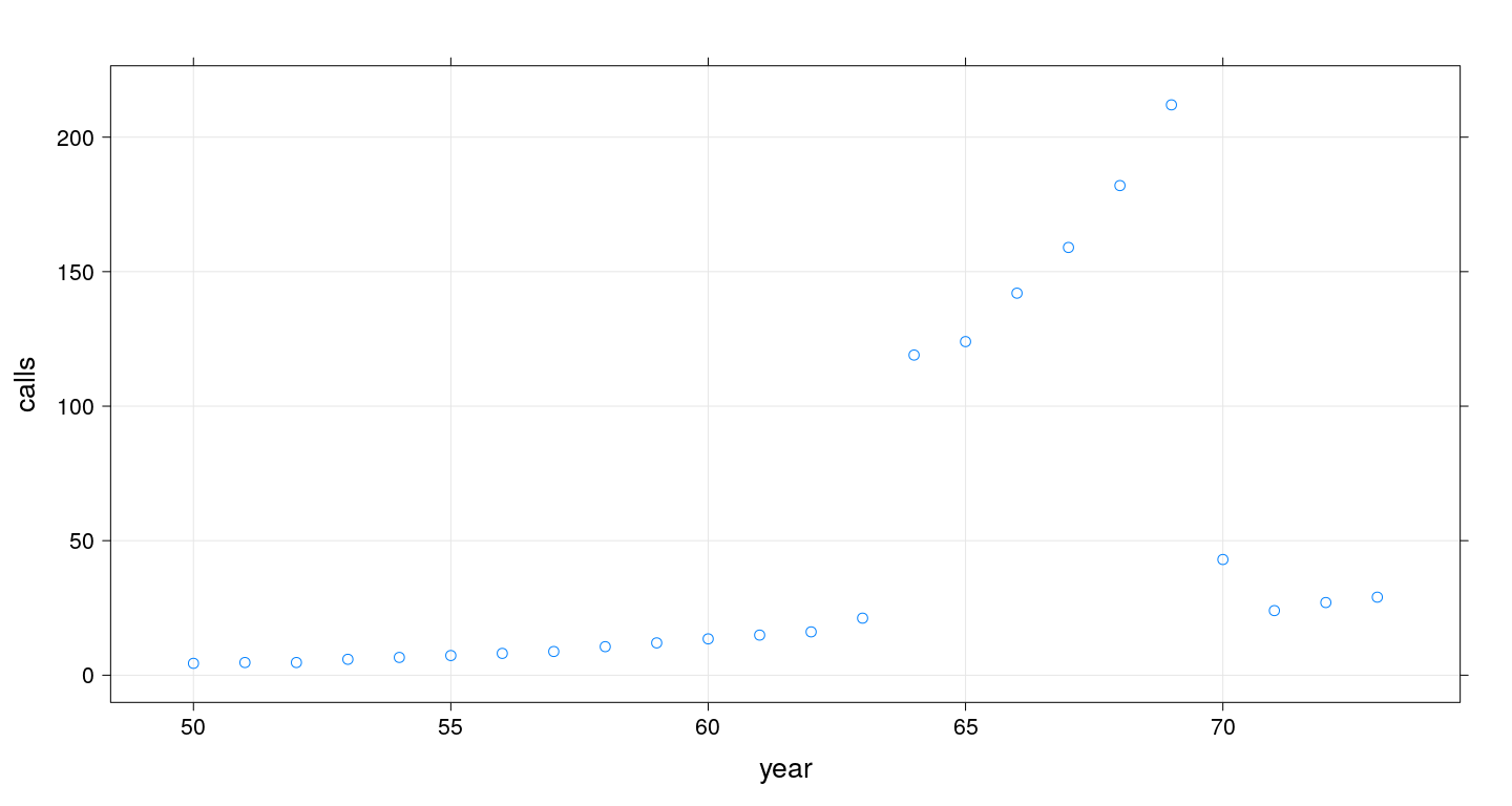
Another example: number of phone calls per year in Belgium
fm2 <- lm(calls ~ year, data = phones)
SAE = function(beta)
{
    with(phones,
         sum(abs(calls - beta[1] - beta[2] * year)))
}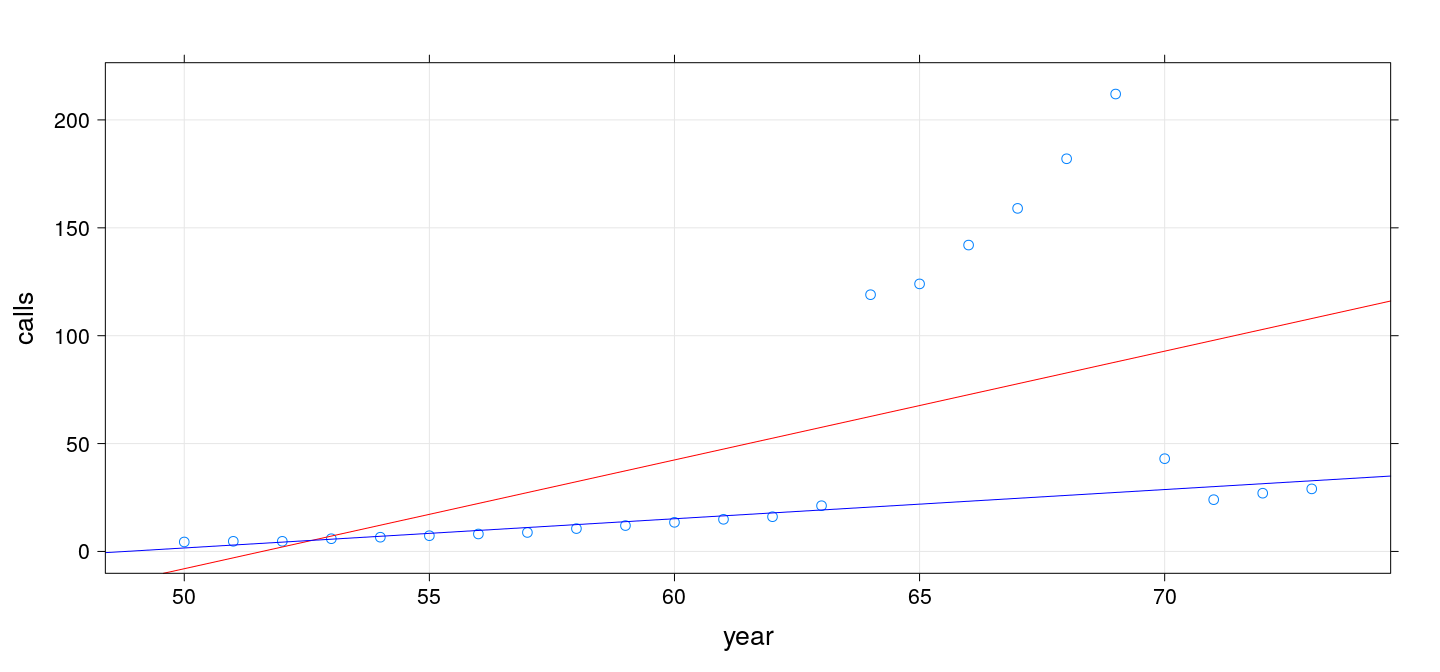
opt = optim(c(0, 0), fn = SAE)(Intercept) year
-260.059246 5.041478 [1] -66.053297 1.353735The two lines are quite different
The second line is an example of robust regression
Another example: number of phone calls per year in Belgium
xyplot(calls ~ year, data = phones, grid = TRUE,
       panel = function(x, y, ...) {
           panel.xyplot(x, y, ...)
           panel.abline(fm2, col = "red") # least squared errors
           panel.abline(opt$par, col = "blue") # least absolute errors
       })
Summary
- Conventional statistical learning focuses on problems that can be “solved” analytically
Numerical solutions are also valid solutions… but potentially difficult to obtain
R makes it easy to obtain numerical solutions and compare with traditional solutions
We will come back to this idea when we next discuss the origins of R
A very brief history of R
What is R?
From its own website:
R is a free software environment for statistical computing and graphics.
It is a GNU project which is similar to the S language and environment which was developed at Bell Laboratories (formerly AT&T, now Lucent Technologies) by John Chambers and colleagues. R can be considered as a different implementation of S.
The origins of S
Developed at Bell Labs (statistics research department) 1970s onwards
Primary goals
Interactivity: Exploratory Data Analysis vs batch mode
Flexibility: Novel vs routine methodology
Practical: For actual use, not (just) academic research
John Chambers received the prestigious ACM Software System Award in 1998
For The S system, which has forever altered how people analyze, visualize, and manipulate data.
The origins of R
Early 1990s: Started as teaching tool by Robert Gentleman & Ross Ihaka at the University of Auckland
1995: Convinced by Martin Mächler to release as Free Software (GPL)
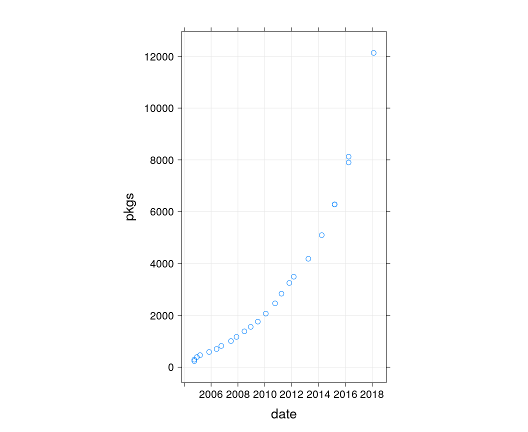
2000: Version 1.0 released
Has since far surpassed S in popularity
Number of R packages on CRAN
Why the success? The user’s perspective
- R is designed for data analysis
- Basic data structures are vectors
- Large collection of statistical functions
- Advanced statistical graphics capabilities
The vast majority of R users use it as a statistical toolbox
R “base” comes with a large suite of statistical modeling and graphics functions
If these are not enough, more than 10000 add-on packages are available
The developer’s perspective
- Easy dissemination of research (through add-on packages)
- Rapid prototyping
- Interfaces to external software
Rapid prototyping
John Chambers, Programming with Data:
S is a programming language and environment for all kinds of computing involving data. It has a simple goal: To turn ideas into software, quickly and faithfully.
A silly example: generate Fibonacci sequence
fibonacci <- function(n) {
    if (n < 2)
        x <- seq(length = n) - 1
    else {
        x <- c(0, 1)
        while (length(x) < n) {
            x <- c(x, sum(tail(x, 2)))
        }
    }
    x
}
fib10 <- fibonacci(10)
fib10
[1] 0 1 1 2 3 5 8 13 21 34Also easy to call C for efficiency
File fib.c:
#include <Rdefines.h>

SEXP fibonacci_c(SEXP nr)
{
    int i, n = INTEGER_VALUE(nr);
    SEXP ans = PROTECT(NEW_INTEGER(n));
    int *x = INTEGER_POINTER(ans);
    x[0] = 0; x[1] = 1;
    for (i = 2; i < n; i++) x[i] = x[i-1] + x[i-2];
    UNPROTECT(1);
    return ans;
}
Compile into shared library:
$ R CMD SHLIB fib.cLoad into R and call:
[1] 0 1 1 2 3 5 8 13 21 34Even easier to call C++ with Rcpp package
File fib.cpp:
#include <Rcpp.h>
using namespace Rcpp;

// [[Rcpp::export]]
NumericVector fibonacci_cpp(int n)
{
    NumericVector x(n);
    x[0] = 0; x[1] = 1;
    for (int i = 2; i < n; i++) x[i] = x[i-1] + x[i-2];
    return x;
}
Compile and call:
[1] 0 1 1 2 3 5 8 13 21 34Rapid prototyping: flexibility and extensibility
Powerful built-in tools
Programming language
Compiled code for efficiency
Another strength: Interfaces
Not all useful software developed by R community
Core open source philosophy: code re-use
Creating interfaces with external software is relatively easy
Example: Keras / TensorFlow
Keras
Deep learning framework based on TensorFlow
R interface through package keras
Example: classify handwritten digits
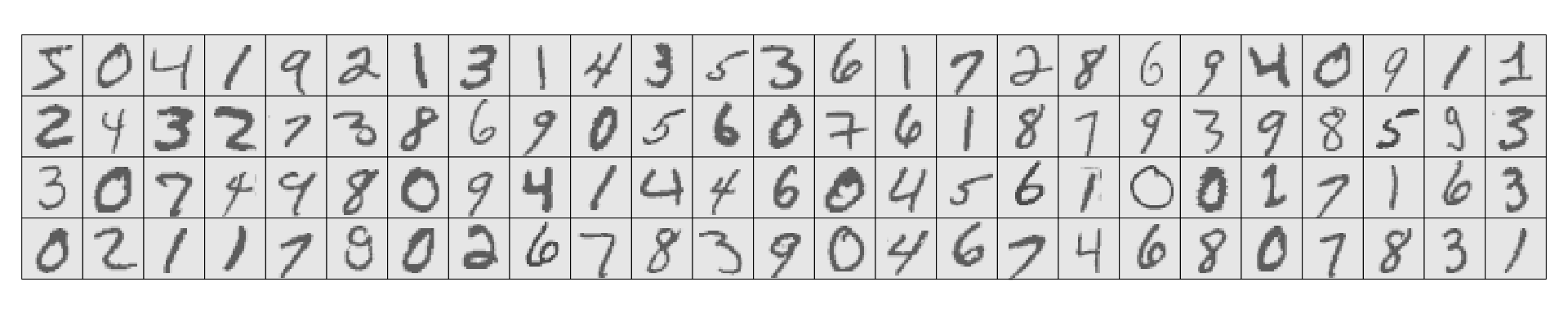
Transform data
- Reshape data (to vector) and rescale
Define model
- A Keras model is a way to organize layers
- Define a sequential model (a linear stack of layers)
model <- keras_model_sequential()
layer_dense(model, units = 256, activation = "relu", input_shape = c(784))
layer_dropout(model, rate = 0.4)
layer_dense(model, units = 128, activation = "relu")
layer_dropout(model, rate = 0.3)
layer_dense(model, units = 10, activation = "softmax")
summary(model)
________________________________________________________________________________________________________________________
Layer (type) Output Shape Param #
========================================================================================================================
dense_1 (Dense) (None, 256) 200960
________________________________________________________________________________________________________________________
dropout_1 (Dropout) (None, 256) 0
________________________________________________________________________________________________________________________
dense_2 (Dense) (None, 128) 32896
________________________________________________________________________________________________________________________
dropout_2 (Dropout) (None, 128) 0
________________________________________________________________________________________________________________________
dense_3 (Dense) (None, 10) 1290
========================================================================================================================
Total params: 235,146
Trainable params: 235,146
Non-trainable params: 0
________________________________________________________________________________________________________________________Compile and train model
Evaluate model
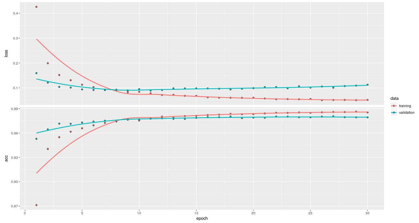
Results on test data
[1] 7 2 1 0 4 1 4 9 5 9 0 6 9 0 1 5 9 7 3 4 [,1] [,2] [,3] [,4] [,5] [,6] [,7] [,8] [,9] [,10]
[1,] 0 0 0 0 0 0 0 1 0 0
[2,] 0 0 1 0 0 0 0 0 0 0
[3,] 0 1 0 0 0 0 0 0 0 0
[4,] 1 0 0 0 0 0 0 0 0 0
[5,] 0 0 0 0 1 0 0 0 0 0
[6,] 0 1 0 0 0 0 0 0 0 0
[7,] 0 0 0 0 1 0 0 0 0 0
[8,] 0 0 0 0 0 0 0 0 0 1
[9,] 0 0 0 0 0 1 0 0 0 0
[10,] 0 0 0 0 0 0 0 0 0 1
[11,] 1 0 0 0 0 0 0 0 0 0
[12,] 0 0 0 0 0 0 1 0 0 0
[13,] 0 0 0 0 0 0 0 0 0 1
[14,] 1 0 0 0 0 0 0 0 0 0
[15,] 0 1 0 0 0 0 0 0 0 0
[16,] 0 0 0 0 0 1 0 0 0 0
[17,] 0 0 0 0 0 0 0 0 0 1
[18,] 0 0 0 0 0 0 0 1 0 0
[19,] 0 0 0 1 0 0 0 0 0 0
[20,] 0 0 0 0 1 0 0 0 0 0Misclassification rate in test data
pred_class    0    1    2    3    4    5    6    7    8    9
         0  971    0    2    0    0    2    4    3    4    5
         1    1 1126    2    0    1    0    3    3    3    2
         2    2    3 1020    4    4    0    0    8    3    1
         3    0    0    0  987    0    2    1    1    5    5
         4    0    0    1    0  957    0    3    0    1    9
         5    2    1    0    9    0  877    3    0    5    4
         6    2    2    0    0    5    5  943    0    1    0
         7    1    0    4    6    2    1    0 1009    3    4
         8    1    3    3    2    1    4    1    1  947    2
9 0 0 0 2 12 1 0 3 2 977[1] 0.9814Another interface: plotly
Plotly: a Javascript library for visualization
R interface provided by the
plotlyR package
More HTML-based applications
Parting comments: reproducible documents
- Creating reports / presentations with numerical analysis is usually a two-step process:
- Do the analysis using a computational software
- Write report in a word processor, copy-pasting results
R makes it very convenient to write “literate documents” that contain both analsyis code and report text
- Basic idea:
- Start with source text file containing code+text
- Transform file by running code and embedding results
- Produces another text file (LaTeX, HTML, markdown)
- Processed further using standard tools
Example: this presentation is created from this source file (R Markdown) using knitr and pandoc
As the source format is markdown, output could also be PDF instead of HTML